LUIZ HENRIQUE DA SILVA ROTTA
Estimation of Submerged Aquatic Vegetation Height
and Distribution in Nova Avanhandava Reservoir (São
Paulo State, Brazil) Using Bio-Optical Modeling
Presidente Prudente
2015
LUIZ HENRIQUE DA SILVA ROTTA
Estimation of Submerged Aquatic Vegetation Height
and Distribution in Nova Avanhandava Reservoir (São
Paulo State, Brazil) Using Bio-Optical Modeling
Thesis for Doctoral Defense Presented to the
Post Graduate Program in Cartographic
Sciences,
Faculty
of
Science
and
Technology – São Paulo State University.
Research Line: Cartography, GIS and Spatial
Analysis.
Advisor: Prof. Dr. Nilton Nobuhiro Imai
Co-Advisor:
Alcantara
Presidente Prudente
2015
Prof.
Dr.
Enner
Herenio
R76e
Rotta, Luiz Henrique da Silva.
Estimation of Submerged Aquatic Vegetation Height and
Distribution in Nova Avanhandava Reservoir (São Paulo State, Brazil)
Using Bio-Optical Modeling / Luiz Henrique da Silva Rotta. Presidente Prudente : [s.n], 2015
124 f. : il.
Orientador: Nilton Nobuhiro Imai
Coorientador: Enner Herenio de Alcântara
Tese (doutorado) - Universidade Estadual Paulista, Faculdade de
Ciências e Tecnologia
Inclui bibliografia
1. Sensoriamento remoto. 2. Modelo bio-óptico. 3. Vegetação
aquática submersa. 4. Cartografia. I. Rotta, Luiz Henrique da Silva
Rotta. II. Nilton Nobuhiro, Imai. III. Alcântara, Enner Herenio de.
Universidade Estadual Paulista. Faculdade de Ciências e Tecnologia.
III. Título.
A Deus.
À minha esposa, pela cumplicidade, apoio
e amor.
Aos meus pais e família por todo carinho
e suporte.
.
AGRADECIMENTOS
Quero expressar meus sinceros agradecimentos a todas as pessoas que
contribuíram para a realização desta pesquisa, cada qual a seu modo. Agradeço em
especial:
A Deus, em primeiro lugar, pelas graças concedidas.
À Simone, esposa dedicada e maravilhosa, pela amizade, carinho,
conselhos, compreensão e todo o imenso amor proporcionado todos os dias, sem o
qual seria impossível desenvolver esta pesquisa.
Aos meus pais, Luiz e Iza, por todo carinho e amor. Aos meus irmãos,
Mone e João e também a toda família, tios, primos e sobrinhos sempre presentes.
À minha sogra e sogro, Lucy e Colemar, pelo acolhimento e carinho, e ao
Lucas, irmão e amigo, sempre disposto a ajudar.
Ao meu orientador, Imai, professor e amigo, pela confiança, ensinamentos
e liberdade no desenvolvimento da tese.
Ao Enner, não somente orientador, mas também um amigo, sempre
disposto a conversar, ensinar e resolver os problemas que surgiram ao longo da
pesquisa.
Ao Deepak Mishra, pela amizade, ensinamentos, e orientação durante o
período do doutorado sanduíche realizado na “University of Georgia”, fundamentais
para os resultados obtidos. Ao departamento de geografia da UGA, pela recepção
no meu doutorado em Athens – GA, Estados Unidos.
Aos professores do departamento de Cartografia, por compartilharem
seus conhecimentos e experiências.
Aos membros da banca de qualificação e de defesa, que contribuíram
com sugestões expressivas.
Aos amigos que me ajudaram muito nos trabalhos de campo, essencial
para o andamento da pesquisa, Ricardo, Ulisses, Rejane, Lino, Renato e em
especial à Fer e Thanan. Nesse sentido agradeço ao Prof. Cláudio do INPE por ter
cedido equipamentos necessários para o levantamento de dados em campo.
Aos amigos do “SRGeoAMA”, pelas discussões científicas e momentos de
descontração e aos amigos do convívio da sala da pós, pelas amizades, festas,
cafezinho e outros momentos.
Ao Conselho Nacional de Desenvolvimento Científico (CNPq) pela bolsa
cedida e pelos recursos dos projetos de pesquisa Universal: CNPq 472131/2012-5 e
CNPq 482605/2013-8, assim como dos projetos FAPESP: 2013/09045-7 e
2012/19821-1. Agradeço também ao CNPq pela bolsa sanduíche, por meio do
projeto CNPq 400881/2013-6.
À UNESP e ao Programa de Pós-Graduação em Ciências Cartográficas,
pela estrutura e auxílio nos trabalhos de campo e participação em eventos
científicos.
Agradeço a todos que não mencionei e que contribuíram direta ou
indiretamente para o desenvolvimento do trabalho.
“A tarefa não é tanto ver aquilo que ninguém
viu, mas pensar o que ninguém ainda
pensou sobre aquilo que todo mundo vê.”
(Arthur Schopenhauer)
RESUMO
Modelos semi-analíticos vêm sendo desenvolvidos para remover a influência da
coluna da água e, com isso, recuperar a resposta do substrato em corpos águas,
com o intuito de estudar alvos submersos. Porém, a maioria desses modelos foram
elaborados para águas oceânicas e costeiras, ou seja, ainda são limitados os
estudos sobre a recuperação da resposta do substrato a partir de sensoriamento
remoto em ambientes aquáticos continentais devido à complexidade desses
ambientes, pois apresentam altas concentrações de constituintes suspensos e
dissolvidos da água, o que dificulta a detecção do sinal do substrato. Os objetivos do
trabalho foram: avaliar a disponibilidade de radiação subaquática na coluna de água
e o total de sólidos suspensos (TSS) no Reservatório de Nova Avanhandava, para
analisar sua influência no desenvolvimento da VAS (Vegetação Aquática Submersa);
recuperar a resposta do substrato e gerar modelos bio-ópticos para estimar a altura
e posição da vegetação aquática submersa no reservatório de Nova Avanhandava; e
finalmente utilizar e avaliar o desempenho dos modelos bio-ópticos por meio de
imagem multiespectral (SPOT-6). Dados hiperespectrais foram coletados com o
radiômetro RAMSES – TriOS. Constatou-se que os estudos sobre disponibilidade de
radiação subaquática medida por meio da atenuação vertical da irradiância
descendente na coluna de água pode auxiliar na compreensão do comportamento
da VAS em reservatórios tropicais e, portanto, contribuir para a sua gestão. A
imagem de satélite, adquirida em 9 de julho de 2013, foi corrigida atmosfericamente
por método empírico. Os dados de profundidade e altura da VAS foram coletados
por ecobatímetro. Com isso, foi possível recuperar a reflectância do substrato por
meio de modelos disponíveis na literatura. Posteriormente, modelos para estimar a
altura da VAS foram calibrados por meio do índice GRVI (Green Red Vegetation
Index) e Slope com as bandas da região do verde e do vermelho. Os modelos com
melhores ajustes foram aplicados na imagem multiespectral para estimar a altura da
VAS em toda área de estudo e, assim, avaliar seu desempenho. O uso do GRVI, na
calibração do modelo para estimar a altura da VAS, se mostrou mais adequado (R² =
0.74 e RMSE = 0.40 m) quando utilizados dados de campo. Porém, ao se utilizar
dados da imagem, a calibração dos modelos foi mais pertinente com o uso do Slope
entre as bandas do verde e vermelho, com R² entre 0.47 e 0.63 e RMSE entre 0.54
e 0.66. Os modelos calibrados foram aplicados na imagem SPOT-6 e obteve-se uma
exatidão global de 53% e índice kappa de 0.34 para o modelo baseado no GRVI. O
modelo utilizado para estimar a presença e ausência de VAS foi altamente eficaz,
com uma exatidão global de 90% e kappa de 0.7. Assim, pela complexidade em se
estudar alvos submersos em água interiores, os resultados trouxeram contribuições
relevantes. Finalmente, observou-se que estudos sobre a disponibilidade de
radiação subaquática por meio da atenuação vertical da radiação na coluna de água
pode ajudar a compreender o comportamento da VAS em reservatórios tropicais e,
portanto, contribuir para sua gestão.
Palavras-Chave: Sensoriamento remoto, modelo bio-óptico, vegetação aquática
submersa, reflectância do substrato, coeficiente de atenuação difusa, Egeria spp.
ABSTRACT
Semi-analytical models have been developed to remove the water column influence
and then retrieve the bottom reflectance in water bodies in order to study submerged
targets. However, the majority of these models were elaborated for oceanic and
coastal waters, in other words, there are still limited studies about the retrieval of the
bottom response from remote sensing in continental aquatic environments. The
reason for that is the complexity of those environments as they present high
concentrations of dissolved and suspended constituents, which make it difficult to
detect the bottom signal. The objectives of this thesis were: to assess the availability
of sub-aquatic radiation in the water column and the total suspended solids
concentration (TSS) in the Nova Avanhandava reservoir in order to analyze their
influence on the SAV (Submerged Aquatic Vegetation) development; to recover the
bottom albedo and generate bio-optical models to estimate the aquatic submerged
vegetation height and position in the Nova Avanhandava reservoir; and finally, to use
and assess the bio-optical models performance by using multi-spectral imagery
(SPOT-6). Hyperspectral data were collected by using the radiometer RAMSES –
TriOS. It was found that studies on subaquatic radiation availability measured by the
vertical attenuation of downwelling irradiance in the water column can aid in
understanding SAV behaviour in tropical reservoirs and, therefore, contribute to its
management. SPOT-6 image, acquired on July the 9th of 2013, was atmospherically
corrected by the empirical line method. The SAV depth and height data were
collected by using the echosounder. Thus, it was possible to recover the bottom
reflectance by using the models available on literature. After, models to estimate the
SAV height were calibrated through GRVI index and Slope with the green and red
regions of the electromagnetic spectrum. The models with better adjustments were
applied on the multispectral image to estimate the SAV height all along the study
area and their performance was assessed. The GRVI usage, when calibrating the
model to estimate the SAV height, presented better results (R² = 0.74 and RMSE =
0.40 m) when used on the field data. However, when using the image data, the
models calibration was more relevant with the usage of Slope between the green and
red bands, presenting a R² between 0.47 and 0.63 and a RMSE between 0.54 and
0.66. The calibrated models were used on the SPOT-6 image to obtain the SAV
height map. The model based on the GRVI presented a global accuracy of 53% and
a kappa index of 0.34. The model calibrated to estimate the occurrence and absence
of SAV was highly effective, presenting a global accuracy of 90% and a kappa of 0.7.
Thus, considering the complexity involved in studying submerged targets into
freshwater, the results made relevant contributions. Finally, it was noted that studies
about the sub-aquatic radiation availability through vertical attenuation of the water
column radiation can help to understand the SAV behavior in tropical reservoirs and
therefore, can be used for their management.
Keywords: Remote sensing, bio-optical model, submerged aquatic vegetation
(SAV), bottom reflectance, diffuse attenuation coefficient, Egeria spp.
LIST OF FIGURES
Figure 1 – Location of the Nova Avanhandava Reservoir in (a) Brazil and (b) São Paulo
state. A true colour satellite image acquired by Landsat OLI sensor (2013-07-04) shows the
reservoir and the surrounding land cover (c). The red rectangle indicates the actual research
site (Bonito River). .............................................................................................................................. 37
Figure 2 – Upstream level of Nova Avanhandava Reservoir between January 2010 and
December 2012. ................................................................................................................................. 39
Figure 3 – Downstream level of Nova Avanhandava Reservoir between January 2010 and
December 2012. ................................................................................................................................. 39
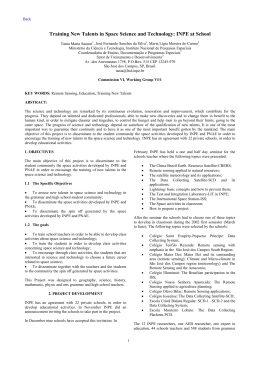
Figure 4 – Average temperature and global radiation monthly in José Bonifácio
meteorological station. ....................................................................................................................... 40
Figure 5 – Average relative humidity and wind speed and precipitation monthly in José
Bonifácio meteorological station. ..................................................................................................... 41
Figure 6 – Submerse aquatic vegetation (Egeria spp.) found in the reservoir of Nova
Avanhandava-SP in October 2012. ................................................................................................. 42
Figure 7 – Sampling stations (black dots), the hydroacustic data collection transects (dotted
red line), and four regions (blue) used in analysis are shown inside the Bonito River (black
outline).................................................................................................................................................. 44
Figure 8 – TriOS optical sensor deployment for Ed measurements above water (a) and below
water (b). .............................................................................................................................................. 45
Figure 9 – Components of the DT-X Echosounder deployed to acquire depth and SAV heigh
data along numerous transects. ....................................................................................................... 47
Figure 10 – Isotropic semivariogram for the SAV height data. A quadratic model was fitted to
the data with nugget, sill, and range values at 0.2, 0.5 and 380, respectively. The fitted model
is represented by the blue line. ........................................................................................................ 49
Figure 11 – Sampling stations with SAV (Green dots) and without SAV (Red dots) and
hydroacoustic data collection transects (Yellow line). .................................................................. 51
Figure 12 – Radiometers (RAMSES/TriOS) used to obtain hyperspectral data....................... 52
Figure 13 – Hyperspectral data collection using TriOS sensor. .................................................. 52
Figure 14 – The AC-S measuring the absorption and attenuation coefficient. ......................... 53
Figure 15 – Backscattering coefficient measured by HydroScat equipment. .......................... 54
Figure 16 – Submerged aquatic vegetation of Bonito River – Nova Avanhandava Reservoir.
............................................................................................................................................................... 55
Figure 17 – Isotropic semivariogram for depth data. A spherical model was fitted to the data
with nugget, sill, and range values at 0, 27 and 480, respectively. The fitted model is
represented by the blue line. ............................................................................................................ 56
Figure 18 – Normalization factor at each scan in P13 showing the variation of illumination
conditions............................................................................................................................................. 57
Figure 19 – Downwelling irradiance before (a) and after (b) normalization and upwelling
radiance before (c) and after (d) normalization in P13 ................................................................. 58
Figure 20 – Diffuse attenuation coefficient based on attenuation and backscattering
coefficients (Kd (a, bb) and based on downwelling irradiance (Kd (Ed)). ..................................... 59
Figure 21 – Relative spectral response of OLI/Landsat 8 (a) and SPOT 6 (b). ........................ 59
Figure 22 – Boxplots for the SAV heights relative to the depths for P01 (a), P02 (b), P03 (c)
and P04 (d). ......................................................................................................................................... 70
Figure 23 – Hyperspectral Ed vertical profile measurements at (a) P01, (b) P02, (c) P03, and
(d) P04 after normalization. ............................................................................................................... 71
Figure 24 – Vertical attenuation of Ed PAR as a function of depth at (a) P01, (b) P02, (c) P03,
and (d) P04. ......................................................................................................................................... 72
Figure 25 – SAV height distribution as function of Percentage Light through the Water (PLW).
............................................................................................................................................................... 73
Figure 26 – SAV height distribution as function of Percentage Light at the Leaf (PLL). ......... 74
Figure 27 – Water body depth as function of the difference between Percent Light through
the Water (PLW) and Percent Light at the Leaf (PLL). ................................................................. 75
Figure 28 – SAV height as function of the difference between Percent Light through the
Water (PLW) and Percent Light at the Leaf (PLL). ....................................................................... 75
Figure 29 – SAV height distribution as a function of depth. The dashed lines represent the
euphotic zone limits (ZEZ) at each point. ....................................................................................... 76
Figure 30 – Three meter long Egeria sp. acquired from the Nova Avanhandava Reservoir
(SP, Brazil) in October 2012. ............................................................................................................ 77
Figure 31 – SAV height map for each region (P01, P02, P03 and P04). .................................. 78
Figure 32 – The Kd (a) and KLu (b) derived from downwelling irradiance (Ed) and upwelling
radiance (Lu), respectively. Dashed line represents the average value. .................................... 79
Figure 33 – Regression to obtain Kd (Green) and Kd (Red) based in green and red
bandwidth according to Palandro et al. (2008). ............................................................................. 80
Figure 34 – Remote sensing reflectance in the sample points. .................................................. 81
Figure 35 – Simulated bands of OLI/Landsat 8 bands in (a) and SPOT 6 in (b) using remote
sensing reflectance of in situ data. .................................................................................................. 82
Figure 36 – Regression between Rrs (Field data) and Digital Number (SPOT-6 image) for
green and red bands. ......................................................................................................................... 82
Figure 37 – Remote sensing reflectance of the bottom retrieved by PAL08 model in (a) and
(c) and irradiance reflectance of the bottom retrieved by DIE03 model in (b) and (d). Average
Kd and KLu derived from in situ data were used in (a) and (b) and a specific Kd and KLu for
each point were used in (c) and (d). ................................................................................................ 84
Figure 38 – Remote sensing reflectance of the bottom retrieved by PAL08 model in (a) and
(c) and irradiance reflectance of the bottom retrieved by DIE03 model in (b) and (d). Average
Kd and KLu derived from in situ data were used on Landsat 8 simulated in (a) and (b) and on
SPOT 6 simulated in (c) and (d)....................................................................................................... 85
Figure 39 – Remote sensing reflectance of the bottom retrieved by PAL08 model in (a) and
(c) and irradiance reflectance of the bottom retrieved by DIE03 model in (b) and (d). Average
KLu derived from in situ data and Kdp were used on Landsat 8 simulated in (a) and (b) and on
SPOT 6 simulated in (c) and (d)....................................................................................................... 86
Figure 40 – Regression between SAV height and GRVI based on remote sensing reflectance
of the bottom retrieved by PAL08. Hyperspectral data: Average Kd derived from in situ data in
(a) and a specific Kd for each point in (b); Landsat 8 simulated: Average Kd derived from in
situ data in (c) and using Kd p in (d); SPOT 6 simulated: Average Kd derived from in situ data
in (e) and using Kd p in (f). Validation for models (e) and (f) are presented in (g) and (h),
respectively.......................................................................................................................................... 87
Figure 41 – Regression between SAV height and Slope based on remote sensing reflectance
of the bottom retrieved by PAL08. Hyperspectral data: Average Kd derived from in situ data in
(a) and a specific Kd for each point in (b); Landsat 8 simulated: Average Kd derived from in
situ data in (c) and using Kd p in (d); SPOT 6 simulated: Average Kd derived from in situ data
in (e) and using Kd p in (f). Validation for models (e) and (f) are presented in (g) and (h),
respectively.......................................................................................................................................... 88
Figure 42 – Regression between SAV height and GRVI based on irradiance reflectance of
the bottom by DIE03. Hyperspectral data: Average Kd and KLu derived from in situ data in (a)
and specific Kd and KLu for each point in (b); Landsat 8 simulated: Average Kd and KLu
derived from in situ data in (c) and using Kd p in (d); SPOT 6 simulated: Average Kd and KLu
derived from in situ data in (e) and using Kd p in (f). Validation for models (e) and (f) are
presented in (g) and (h), respectively. ............................................................................................. 89
Figure 43 – Regression between SAV height and Slope [Rb(Green) : Rb(Red)] based on
irradiance reflectance of the bottom by DIE03. Hyperspectral data: Average Kd and KLu
derived from in situ data in (a) and specific Kd and KLu for each point in (b); Landsat 8
simulated: Average Kd and KLu derived from in situ data in (c) and using Kd p in (d); SPOT 6
simulated: Average Kd and KLu derived from in situ data in (e) and using Kd p in (f). Validation
for models (e) and (f) are presented in (g) and (h), respectively. ............................................... 90
Figure 44 – Regression between SAV height and GRVI of SPOT simulated based on
irradiance reflectance of the bottom by DIE03 and average Kd and KLu derived from in situ
data. ...................................................................................................................................................... 91
Figure 45 – Regression between SAV height and GRVI based on remote sensing
reflectance of the bottom by PAL08 in (a) and (b) and based on irradiance reflectance of the
bottom by DIE03 in (e) and (f). Average Kd and KLu derived from in situ data were used in (a)
and (e); Kd p was used in (b) and (f). (j) and (l). The validation for each model is under itself.
Validation for models (a), (b), (e) and (f) are presented in (c), (d), (g) and (h), respectively. . 92
Figure 46 – Regression between SAV height and Slope [(Green):(Red)] based on remote
sensing reflectance of the bottom by PAL08 in (a) and (b) and based on irradiance
reflectance of the bottom by DIE03 in (e) and (f). Average Kd and KLu derived from in situ
data were used in (a) and (e); Kd p was used in (b) and (f). (j) and (l). The validation for each
model is under itself. Validation for models (a), (b), (e) and (f) are presented in (c), (d), (g)
and (h), respectively. .......................................................................................................................... 93
Figure 47 – Logarithmical regression between SAV height and Slope [(Green):(Red)] of
SPOT image based on remote sensing reflectance of the bottom by PAL08 Average Kd
derived from in situ data were used in (a) and Kd p was used in (b). Validation for models (a)
and (b) are shown in (c) and (d), respectively. .............................................................................. 94
Figure 48 – Logarithmical regression between SAV height and Slope [(Green):(Red)] of
SPOT image based on remote sensing reflectance of the bottom by DIE03. Average Kd and
KLu derived from in situ data were used in (a) and Kd p was used in (b). Validation for models
(a) and (b) are shown in (c) and (d), respectively.......................................................................... 95
Figure 49 – Bathimetry of Bonito River – Nova Avanhandava Reservoir.................................. 96
Figure 50 – Map of the occurrence of Submerse Aquatic Vegetation. ...................................... 98
Figure 51 – SAV height estimation using SAV Model 1 (Equation (30)). Bottom retrieved by
DIE03.................................................................................................................................................... 99
Figure 52 – SAV height estimation using SAV Model 2 (Equation (31)) in (a) and SAV Model
3 (Equation (32)) in (b). Bottom retrieved by PAL08. ................................................................. 100
Figure 53 – S SAV height estimation using SAV Model 4 (Equation (33)) in (a) and SAV
Model 5 (Equation (34)) in (b). Bottom retrieved by DIE03........................................................ 101
Figure 54 – Histogram and descriptive statistic of SAV height in Bonito River. ..................... 105
Figure 55 – SAV height estimation using SAV Model 1. Bottom retrieved by DIE03. ........... 110
LIST OF TABLES
Table 1 – Primary characteristics of the Nova Avanhandava Reservoir. .................................. 38
Table 2 – Depth for each sample station ........................................................................................ 51
Table 3 – Multispectral bands of OLI/Landsat 8 and SPOT 6. .................................................... 60
Table 4 – SPOT-6 image characteristics. ....................................................................................... 61
Table 5 – Main characteristics of each model used on the mapping of SAV. ........................... 64
Table 6 – Suspended solids concentration and depths at the sampling locations. TSS: total
suspended solids, FSS: fixed suspended solids, and VSS: volatile suspended solids. ......... 67
Table 7 – Descriptive statistics for the SAV heights at different depths and sampling stations.
N is the number of readings acquired from the echosounder transects, Freq. is the frequency
for N at each depth, SD is the standard deviation, Min, Median, and Max are the minimum,
median, and maximum values for each dataset, and Q1 and Q3 are the first and third
quartiles, respectively. ....................................................................................................................... 68
Table 8 – Diffuse attenuation coefficient (Kd) of Photosynthetically Active Radiation (PAR)
and the euphotic zone depth (ZEZ) for each point.......................................................................... 73
Table 9 – Confusion matrix of the SAV height estimation map using SAV Model 1 based on
Reflectance retrieved by DIE03. .................................................................................................... 102
Table 10 – Confusion matrix of the SAV height estimation map using SAV Model 2 based on
Reflectance retrieved by PAL08. ................................................................................................... 102
Table 11 – Confusion matrix of the SAV height estimation map using SAV Model 3 based on
Reflectance retrieved by PAL08. ................................................................................................... 103
Table 12 – Confusion matrix of the SAV height estimation map using SAV Model 4 based on
Reflectance retrieved by DIE03. .................................................................................................... 103
Table 13 – Confusion matrix of the SAV height estimation map using SAV Model 5 based on
Reflectance retrieved by DIE03. .................................................................................................... 104
Table 14 – Confusion matrix of the SAV height estimation map using SAV Model 1 based on
Reflectance retrieved by DIE03. .................................................................................................... 106
Table 15 – Confusion matrix of the SAV height estimation map using SAV Model 2 based on
Reflectance retrieved by PAL08. ................................................................................................... 106
Table 16 – Confusion matrix of the SAV height estimation map using SAV Model 3 based on
Reflectance retrieved by PAL08. ................................................................................................... 107
Table 17 – Confusion matrix of the SAV height estimation map using SAV Model 4 based on
Reflectance retrieved by DIE03. .................................................................................................... 107
Table 18 – Confusion matrix of the SAV height estimation map using SAV Model 5 based on
Reflectance retrieved by DIE03. .................................................................................................... 108
Table 19 – Confusion matrix of SAV distribution map. Reflectance of the bottom was
retrieved by DIE03............................................................................................................................ 111
LIST OF ABBREVIATIONS AND ACRONYMS
{Dd} – Vertically averaged downwelling distribution function
a – Absorption coefficient
AC-S – In-situ spectrophotometer for absorption and attenuation coefficients
AOP – Apparent Optical Properties
ASCII - American Standard Code for Information Interchange
bb – Backscattering coefficient
Bde – Total dry weight of epiphytic materials
Be – Epiphyte biomass
C: pixel-independent constant
DIE03 – Model to retrieve the bottom as described in Dierssen et al. (2003)
DN – Digital Number
DuB – The path-elongation factors for photons scattered by the bottom
DuC – The path-elongation factors for photons scattered by the water column
Ed – Downwelling irradiance
Ed PAR – Integration of the Ed between 400 nm and 700 nm
Ed PAR (ZEZ) – Downwelling irradiance of PAR at the euphotic zone depth limit ZEZ –
Euphotic zone depth limit
Es – Incident surface irradiance
Eu/Ed – Irradiance reflectance
Fi – Spectral immersion coefficient
FLAASH – Fast Line-of-sight Atmospheric Analysis of Spectral Hypercubes
FSS – Fixed Suspended Solids
GPS - Global Positioning System
GRVI – Green-Red Vegetation Index
H – Depth
HydroScat – Backscattering Sensor
INMET (Instituto Nacional de Meteorologia) – National Institute of Meteorology
IOP – Inherent Optical Properties
K – Attenuation coefficient
Kd – Vertical diffuse attenuation coefficient of downwelling irradiance (Ed)
Kd P – Diffuse attenuation coefficient as in Palandro et al. (2008)
Ke – Biomass-specific epiphytic light attenuation coefficient
KLu – Vertical diffuse attenuation coefficient of upwelling radiance (Lu)
KuB – Vertical average diffuse coefficient of attenuation for upwelling irradiance of the
bottom
KuC – Vertical average diffuse coefficient of attenuation for upwelling irradiance of the
water column scattering
LEGAL (Linguagem Espacial para Geoprocessamento Algébrico) – Spacial
Language for Algebric Geoprocessing
Lp – Radiance from reference panel
Lu – Upwelling radiance
MODTRAN – MODerate spectral resolution atmospheric TRANsmittance algorithm
and computer model
n – Refractive index of water relative to air (1.33)
NDVI – Normalized Difference Vegetation Index
NF – Normalization factor
OLI - Operational Land Imager
PAL08 – Model to retrieve the bottom as described in Palandro et al. (2008)
PAR – Photosynthetically Active Radiation
PLL – Percent Light at the Leaf
PLW – Percent Light through the Water
Q – Ratio of upwelling irradiance and upwelling radiance (Eu/Lu)
Qb – Ratio of upwelling irradiance and upwelling radiance (Eu/Lu)
R² – coefficient of determination
Rb – Irradiance reflectance of the bottom
Rdp – Irradiance reflectance of deep water
Rrs – Above-water remote sensing reflectance
rrs – Remote sensing reflectance just below the water surface
Rrsb – Remote sensing reflectance above surface from the bottom
rrsb – Remote sensing reflectance just below the water surface from the bottom
Rrsc – Remote sensing reflectance above surface from water column
rrsc – Remote sensing reflectance just below the water surface from water column
rrsdp – Remote sensing reflectance just below the water surface for optically deep
water
SAV – Submerged Aquatic Vegetation
SPOT (Satellite Pour l’Observation de la Terre) – Satellite for observation of Earth
SPRING (Sistema de Processamento de Informações Geográficas) – Geographic
Information Processing System
Sus – Subsurface upwelling signal
SusB – Upwelling signal above the bottom.
Susdp – Signal in deep water
t – Transmittance at air-water interface (0.98)
TSS – Total Suspended Solids
UGRHI (Unidades de Gerenciamento de Recursos Hídricos) – Water Resources
Management Unit
VSS – Volatile Suspended Solids
Z – Depth
θϑ – Subsurface sensor viewing angle from nadir
θω – Subsurface solar zenith angle
ρ – Bottom albedo
ρp – Stands for the reflectance of reference panel
CONTENTS
1.
INTRODUCTION ........................................................................................................................ 22
1.1 Motivation ................................................................................................................................ 24
1.2. Hypothesis ............................................................................................................................. 26
1.3 Objectives ................................................................................................................................ 26
1.4 Structure of thesis ................................................................................................................. 26
2.
REVIEW ....................................................................................................................................... 27
2.1 Aquatic vegetation ................................................................................................................ 27
2.2 The relationship between SAV and radiation availability ........................................... 28
2.3 Optical properties of water.................................................................................................. 29
2.3.1 Diffuse attenuation coefficient.................................................................................... 30
2.4 Remote sensing reflectance ............................................................................................... 33
2.4.1 Retrieving bottom reflectance .................................................................................... 33
3.
STUDY SITE ............................................................................................................................... 37
4.
MATERIAL AND METHOD ...................................................................................................... 43
4.1 First field campaign .............................................................................................................. 43
4.1.1 Suspended Solids Measurement ............................................................................... 45
4.1.2 Hyperspectral downwelling irradiance ..................................................................... 45
4.1.2.1 Diffuse attenuation coefficient (Kd) .................................................................... 46
4.1.3 Echosounder data .......................................................................................................... 46
4.1.3.1 SAV Height Interpolation....................................................................................... 48
4.1.4 The relationship between SAV and radiation availability .................................... 49
4.2 Second field campaign......................................................................................................... 50
4.2.1 Apparent optical proprieties........................................................................................ 52
4.2.2 Inherent optical proprieties ......................................................................................... 53
4.2.3 Echosounder data .......................................................................................................... 55
4.2.4 Diffuse attenuation coefficient (Kd) ........................................................................... 57
4.2.5 In situ remote sensing reflectance ............................................................................ 59
4.2.6 Satellite data .................................................................................................................... 61
4.2.6.1 Atmospheric correction ........................................................................................ 61
4.2.7 Bottom reflectance ......................................................................................................... 62
4.2.8 Model calibration and validation for estimative of SAV height .......................... 63
4.2.9 SAV height mapping using SPOT-6 image .............................................................. 64
4.2.9.1 SAV height map validation ................................................................................... 65
5. RESULTS AND DISCUSSION .................................................................................................... 67
5.1 Relationship between radiation availability and submerged aquatic vegetation
characteristics............................................................................................................................... 67
5.1.1 Suspended solids........................................................................................................... 67
5.1.2 SAV height statistics ..................................................................................................... 68
5.1.3 Hyperspectral analysis ................................................................................................. 71
5.2 Bio-optical models to estimate the SAV height ............................................................. 79
5.2.1 Diffuse attenuation coefficients ................................................................................. 79
5.2.2 Remote sensing reflectance ........................................................................................ 80
5.2.2.1 Satellite bands simulation .................................................................................... 81
5.2.3 Atmospheric correction of satellite data .................................................................. 82
5.2.4 Retrieved bottom reflectance ...................................................................................... 83
5.2.5 SAV models based on in situ data ............................................................................. 86
5.2.6 SAV models based on satellite data .......................................................................... 92
5.3 Submerged aquatic vegetation height mapping using spot-6 satellite image ...... 95
5.3.1 River Depth ...................................................................................................................... 96
5.3.2 Submerged Aquatic Vegetation Height and Distribution .................................... 97
5.3.3 SAV Map Validation ..................................................................................................... 101
6. CONCLUSION ............................................................................................................................. 112
22
1.
INTRODUCTION
Nearly 90% of the area flooded by dams in Brazil is a consequence of the
hydrologic installations established in the last 40 years in the South Western, Centre
Western and Southern regions (ARAÚJO-LIMA et al., 1995). Several dams were
constructed throughout Brazil for electrical power generation following its industrial
and socio-economic development, which yielded many artificial lake ecosystems
(ESTEVES, 2011). Reservoirs and natural lakes differ in significant ways; however,
there are many functional similarities between these ecosystems (WETZEL, 2001).
The processes and functions that are common to reservoirs and lakes include
internal mixing, gas exchange across air-water interface, redox reactions, nutrient
uptake, predator-prey interactions, and primary production. The main primary
producers in reservoirs are the same as in rivers and lakes and primarily include
phytoplankton, photoautotrophic bacteria, periphytic algae, and macrophytes (both
rooted, floating, emerged and submerged) (TUNDISI and TUNDISI, 2008).
Macrophytes are important in the biodiversity-support functioning of freshwater
systems: it is vital for many animal communities (such as aquatic invertebrates, fish
and aquatic birds), change the water and sediment physic-chemistry, influence the
nutrient cycling, can be food for invertebrates and vertebrates, and change the
spatial structure of the waterscape by increasing habitat complexity (THOMAZ et al.,
2008). Submerged macrophytes occupy key interfaces in aquatic ecosystems, so
they have major effects on productivity and biogeochemical cycles in fresh water
(CARPENDER and LODGE, 1986). Egeria densa and Egeria najas are among the
primary species of submerged macrophytes found in Brazilian reservoirs (THOMAZ
and BINI, 1998; CAVENAGHI et al., 2003; MARCONDES et al., 2003; BINI and
THOMAZ, 2005).
Several factors impact primary productivity of the aquatic macrophytes, such
as temperature, radiation availability, stream velocity, water level variation, nutrient
concentration, competition, and inorganic carbon (CAFFREY et al., 2007; CAMARGO
et al., 2003; BIUDES and CAMARGO, 2008). However, radiation availability is the
primary limiting factor for submerged aquatic macrophytes (SCHWARZ et al., 2002;
HAVENS, 2003; TAVECHIO and THOMAZ, 2003; THOMAZ, 2006; RODRIGUES
and THOMAZ, 2010; KIRK, 2011). When traversing the water column, the radiation
changes primarily due to the concentration of materials both in solution and
23
suspension (ESTEVES, 2011). Most of these materials in the water column absorb
and scatter radiation and are referred to as “optically active constituents”. Studies on
five Tietê River reservoirs in Brazil showed that suspended solids have a great effect
on light transmission through the water column and, thus, determine the development
of submerged aquatic vegetation (SAV) (CAVENAGHI et al., 2003). Therefore, it is
important assess the spatial distribution of suspended solid concentration and, after
that, its influence on radiation availability and SAV productivity.
It is known the importance of radiation availability for growth and maintenance
of submerged aquatic vegetation, but studies are needed to explain in detail the
relationship between SAV and radiation. Thus, the use of optical parameters in this
analysis may contribute significantly to understand better the SAV behavior in
Brazilian reservoirs. Further, it is necessary to know the spatial distribution of
submerged macrophyte to aid in water body management. Thus, different techniques
to map this vegetation have been used (WATANABE et al., 2013; VAHTMÄE and
KUTSER, 2013). In addition of SAV mapping, the photosynthetically active radiation
behaviour along the water column should be studied to assess subaquatic radiation
availability.
The constituents dissolved and suspended in the water column, named
“optically active”, cause the radiation, when penetrating into the water, to be
absorbed and scattered. According to Kirk (2011), the absorption and scattering
properties of light in aquatic environment, in any wave length, are specified in terms
of absorption coefficient, scattering coefficient and volume scattering function. They
are the Inherent Optical Properties - IOP, for and their magnitude depends only on
the aquatic environment and not on the geometrical structure of the light field.
Empirical models are widely used in the inference of optically active
components on water bodies through remote sensing. Rotta et al. (2009) used
multispectral images and in situ measurements to generate a regression model to
infer the spatial distribution of suspended solids in the floodplain of upper Paraná
River. Ferreira et al. (2009), through empirically generated model, performed the
spatial inference of pigments in suspension through multispectral images. Rudorff et
al. (2007) compared the performance of empirical algorithms to estimate the
concentration of chlorophyll-a by remote sensing data and in situ measurements.
Analytical or semi-analytical models incorporate, besides the Inherent Optical
Properties, the Apparent Optical Properties. Apparent Optical Properties (AOP) are
24
dependent on both the environment and the directional structure of the ambient light
field. The semi-analytical model can provide response of the optically active
components and the bottom. Also, it is possible to detect the submersed
macrophytes in water bodies of water, as this vegetation has been causing many
problems in reservoirs.
In the reservoirs built until nowadays, either for storing water or for hydropower
production, water quality is already sufficiently compromised since the filling, i.e. the
eutrophication level is sufficient to support significant growth of submergsed
macrophytes, floating and marginal (PITELLI, 2006).
Marcondes et al. (2003) in their study, showed that in the rainy period, the
increase of the reservoir flow causes the fragmentation of submerged aquatic plants
and leads this vegetation to be dragged by the reservoir toward the hydroelectric
plant, hampering navigation, fishing, capture and leisure. Those plants generally
accumulate in the guardrails of the water intake of generating units causing clogging
of the grids and, consequently, decrease the uptake of water and this causes
turbines' power oscillation. The greater pressure on the grids may inflict deformation
or breakage of them, making it necessary to interrupt the operation of the generating
unit to replace the damaged grids.
In fact, the remote sensing studies developed to estimate optically active
components
in
Brazil
still
focus
on
empirical
approach.
However,
the
parameterization of semi-analytical models and their adaptation in albedo estimation
models in optically shallow water reservoirs of São Paulo power plants would be a
valuable contribution, allowing the mapping of SAV.
1.1 Motivation
The importance of radiation availability is known for growth and maintenance
of submerged aquatic vegetation, but studies are needed to explain in detail the
relationship between SAV and radiation. Thus, the use of optical parameters in this
analysis may contribute significantly to understand better the SAV behavior in
Brazilian reservoirs. Further, it is necessary to know the spatial distribution of
submerged macrophyte to aid in water body management. Different techniques to
detect this vegetation have been used (WATANABE et al., 2013; VAHTMÄE and
KUTSER, 2013). In addition of SAV mapping, the photosynthetically active radiation
25
behavior along the water column must be studied to assess subaquatic radiation
availability.
The calculation of the spatial distribution of SAV is a costly task currently,
when performed with data from field surveys. The procedures involved in such
calculation require long time and therefore the mapping of SAV is impracticable,
especially in large reservoirs. However, this alternative is very common, because it
allows the researcher to create the inventory and also identify the vegetation
(POMPÊO and MOSCHINI-CARLOS, 2003). Another option is based on calculations
with sonars that produce bathymetry, density and height data of the SAV (VALLEY
and DRAKE, 2005). However, those hydroacoustic techniques demand long time if
conducted with few boats.
An alternative for detecting SAV is the use of remote sensing data. According
Dekker et al. (2001), if the water column is sufficiently transparent and the bottom is
at a depth where enough quantity reaches the bottom and it is reflected back out of
the water body, so, it is possible to produce maps of macrophytes, macro-algae,
shoals, coral reefs etc.
(DEKKER et al., 2001).The spectral response to of the
bottom in optically shallow water at the ocean shore was estimated by Lee et al.
(2007). This approach allows the mapping of corals based on hyperspectral images.
Other studies show that inverse models based on the Radiative Transfer Theory in
water bodies can be adapted to estimate the response of the bottom or even to
estimate the height of the water column (GIARDINO et al., 2012; BRANDO et al.
2009; ALBERT and MOBLEY, 2003; DEKKER et al., 2001; LEE et al., 1998, 1999
and 2001).
Multispectral images have been used to study benthic habitats. Mishra et al.
(2006) used Quickbird multispectral data to benthic habitat mapping in tropical
marine environments. Mumby et al. (2004) indicated the possibility to study reef
geomorphology, location of shallow reefal areas, reef community (<5 classes),
bathymetry and coastal land use by Landsat and SPOT images.
There are some methods to retrieve the bottom response from reflectance
(e.g., LEE et al., 1994; MARITORENA et al., 1994; LEE et al., 1999; LEE AND
CARDER, 2002) which presented suitable results and could be tested to the Nova
Avanhandava Reservoir. Palandro et al. (2008) used Kd to remove water-column
attenuation effect from Rrs, obtaining the remote sensing reflectance of the bottom
(Rrsb). Dierssen et al. (2003) presented a method derived of Beer’s Law to retrieve
26
the irradiance reflectance (Eu/Ed) of the bottom (Rb). After retrieving the response of
the bottom it is possible to extract information such as localization and height of the
SAV in the studied reservoir.
1.2. Hypothesis
This study is based on the hypothesis that from multispectral data and based
on the radiative transference theory in the water column it is possible to retrieve the
bottom reflectance by remote sensing, to identify and estimate the height of the
submerged aquatic vegetation present in the reservoir.
1.3 Objectives
The objectives of the study are:
•
To assess the subaquatic radiation availability in the water column and
the total suspended solid (TSS) concentration in the Nova Avanhandava Reservoir
and analyze its influence on SAV initiation and development;
•
To retrieve the bottom response and generate bio-optical models to
estimate the height and the position of submerged aquatic vegetation in the Nova
Avanhandava reservoir;
•
To use and evaluate the performance of bio-optical models of the
generation of maps of the distribution and SAV height through multispectral image –
SPOT-6.
1.4 Structure of thesis
This thesis consists of six chapters and three appendices. Chapter 1 holds the
introduction and Chapter 2 the review on the relevant issues of the study. The
characterization of the study area is done on Chapter 3. The Chapter 4 brings
materials and methods and Chapter 5 the results and discussion. Finally, the
conclusions are presented on Chapter 6.
27
2.
REVIEW
2.1 Aquatic vegetation
Aquatic plants can be grouped into three main assemblages: Emergent –
rooted at the bottom and projecting out of the water for part of their length; Floating –
which wholly or in part float on the water surface; and Submerged – they are
continuously submerged (WETCH, 1952). They also can be divided in: rooted
submerged – plants that grow completely submerged and are rooted into the
sediment; free-floating – plants that float on or under the water surface; emergent –
plants rooted in the sediment with foliage extending into the air; and floating-leaved –
plants rooted in the sediment with leaves floating on the water surface. Epiphytes
(plants growing over other aquatic macrophytes) and amphibious (plants that live
most of their life in saturated soils, but not necessarily in water) are additional life
forms that have been proposed (THOMAZ et al., 2008).
In Brazil, the submerged aquatic vegetation (SAV) with the highest expression
in power generation reservoirs and rural dams are Egeria densa and Egeria najas.
Among the damage caused by excessive growth of this plant is the favoring for
disease vectors breeding. The marketing of E. densa e E. najas as ornamental plant
for aquariums made possible its spread to various parts of the world (MARTINS et
al., 2003).
Thomaz (2006) found that in a chain of the Tietê River reservoirs, the highest
occurrences of submerged plants were found in reservoir downstream of Três Irmãos
- the last reservoir of the series. But the predominance of floating macrophytes
occurred in Barra Bonita, the first of the series in middle Tietê River. Considering the
reservoirs individually (research mainly developed in Itaipu and Rosana reservoirs in
the Paraná and Paranapanema rivers, respectively) some factors that explained the
distribution of aquatic vegetation were level of water, nutrients, underwater radiation,
fetch (way to assess the effects of wind ) and slope.
Furthermore, Thomaz (2006) found that underwater radiation has been an
extremely important variable to explain the submerged plants distribution patterns
within the same reservoir. Study in Rosana Reservoir showed that the different
distribution of E. densa and E. najas can be associated with that factor, since the
former species predominates in the lake region, while the latter, in the intermediate
28
region. This trend was also observed in the Itaipu reservoir, where the probability of
E. najas is higher in places with less water transparency in comparison to E. densa.
2.2 The relationship between SAV and radiation availability
The hyperspectral downwelling irradiance data can be used to compute the
vertical attenuation coefficient (Kd) and euphotic zone depth. These parameters can
analyze the influence of radiation availability on SAV incidence and development. In
addition, two optical parameters which act as proxy to radiation availability in SAV
habitats can be computed: (1) Percent Light through the Water (PLW) and (2)
Percent Light at the Leaf (PLL). PLW is a measure of the light transmitted through
the water column to the depth of SAV growth, and PLL considers the additional light
attenuation by epiphytic materials (KEMP et al., 2004).
PLW is calculated as an exponential relationship to depth of SAV growth (Z)
and attenuation coefficient (Kd) (Equation (1)). PLL (Equation (2)) is calculated using
PLW and variables derived from numerical and empirical relationships, Be, epiphyte
biomass and Ke, biomass-specific epiphytic light attenuation coefficient (KEMP et al.
2000).
PLW  100  e  Kd Z
(1)
PLL  PLW  e  KeBe
(2)
K e 0.07  0.32  ( Be / Bde ) 0.88
(3)
where, Bde is the total dry weight of epiphytic materials. A significant relationship (r 2 =
0.85) was observed among Bde, Be and TSS in a set of studies in experimental ponds
(TWILLEY et al., 1985):
Bde  0.107  TSS  0.832  Be
(4)
29
2.3 Optical properties of water
The water color is a complex optical characteristic and it is influenced by the
absorption processes, scattering and emission by the water column and reflectance
by the bottom (DEKKER et al., 2001).
According to Kirk (2011), radiation, when penetrating into the water, may be
absorbed or scattered. The absorption or scattering properties of light in the aquatic
environment, at any wave length, are specified in terms of absorption coefficient,
spread coefficient and volumetric spread function. They are the Inherent Optical
Properties – IOPs, for their magnitude depends solely on the aquatic environment
and not on the geometrical structure of the light field. The two fundamental Inherent
Optical Properties - coefficient of absorption and scattering - can be defined in terms
of the behavior of a parallel beam of light incident on a thin layer of the medium.
Apparent Optical Properties – AOP, are dependent both on the medium and
on the directional structure of the ambient light field. An ideal AOP changes slightly
with external environmental changes, but, it modifies a water body to another
sufficiently, which makes it useful in the characterization of different optical properties
of two water bodies. Unlike the IOP, the AOP cannot be measured in water samples
as they depend on the distribution of environmental radiance found in the water body
(MOBLEY, 1994).
For the mapping of the bottom, the relationship between the optical properties
and the concentration of the particles of the water column should be known as well
as the optical properties of the bottom. If the inherent optical properties of the
optically active components are sufficiently well characterized, their contributions for
the color of the water column can be discriminated and their content quantified. Due
to the fact that the radiation reflected by the water depends on the quality and the
specific optical properties of one or more constituents of the water, its color carries
spectral information on the concentration of some parameters of water quality and
possibly of the bottom (DEKKER et al., 2001).
For the retrieval of different constituents of the water and the bottom cover,
using the signaling of hyperspectral remote sensing, there is a group of inversion
methods available. It ranges from the frequently used, although less precise
regression methods, up to the inversion models based on physical principles or
inversion methods. If the water column is sufficiently transparent and the bottom is at
30
a depth where enough quantity reaches the bottom and it is reflected back out of the
water body, so, it is possible to produce maps of macrophytes, macro-algae, shoals,
coral reefs etc. (DEKKER et al., 2001).
2.3.1 Diffuse attenuation coefficient
Cloud cover variability can cause variations in incident surface irradiance, Es
(z, λ). So, it is strongly recommended that all scans be normalized to a specific scan
(Mueller, 2003). The normalization factor NF (z, λ) for each scan can be calculated
as:
(
)
, (
) -
(5)
, ( ) -
where,
, (
) -: is the downwelling irradiance measured at the first scan at time t(0-) on
the boat.
, ( ) -: is the downwelling irradiance measured at time t(z) on the boat.
A normalization factor greater than 1 indicate lower irradiance, as clouds
shadow, and values less than 1 indicate brighter conditions (MISHRA et al., 2005).
To normalize the spectral data and eliminate the noise due to change in illumination,
the Equation (6) can be used for the downwelling irradiance and Equation (7) for
upwelling radiance.
(
)
(
)
(
)
(6)
(
)
(
)
(
)
(7)
Diffuse attenuation coefficient is the parameter that controls the propagation of
light through water. Characterizing the water column, Kd is important because it can
quantify the presence of light in different depths and determine the euphotic zone
(MISHRA et al., 2005). Vertical diffuse attenuation coefficient (Kd) can be defined as
the exponential decrease in ambient irradiance as a function of depth (KIRK, 2011).
31
Radiances and Irradiances decrease exponentially with depth, therefore the
downwelling irradiance Ed (z, λ) is (MOBLEY, 1994):
(
)
(
)
(
)
(8)
Isolating the variable Kd yields the following:
Kd 
ln E d (0)  ln E d ( z )
Z
(9)
The same way of Equation (8), it is possible to calculate the attenuation
coefficient of upwelling radiance Lu (z; λ) (MUELLER et al., 2003):
(
)
(
)
(
)
(10)
The Kd also can be calculated using the inherent optical properties of the
water. The Kd can be simply expressed as function of the absorption (a) and
backscattering coefficients (bb) (SATHYENDRANATH et al., 1989; MOBLEY, 1994;
LEE et al., 2005):
(
)
(11)
where,
is the solar zenith angle just below the surface.
Palandro et al. (2008) calculated the Kd of a water body using only the spectral
images from satellite and the depth. This diffusion attenuation coefficient will be
described as Kd P.
( )
where,
Kd P: diffuse attenuation coefficient in Palandro’s methodology;
(12)
32
Rrs(z): above-water remote sensing reflectance for a pixel with bottom depth Z;
C: pixel-independent constant.
Photosynthetically Active Radiation (PAR) comprehends the spectrum range
of solar radiation from 400 nm to 700 nm.
So, The Ed PAR can be calculated
integrating the Ed between 400 nm and 700 nm. Based on Equation (8), Ed PAR can
be obtained:
( )
(
( )
)
(13)
The illuminated portion of the water column, the euphotic zone, can vary from
a few centimeters to tens of meters. Euphotic zone is the region in a body of water
with sufficient PAR to sustain photosynthesis (KIRK, 2011).The euphotic zone lower
limit is typically the depth where the photosynthetically active radiation corresponds
to 1% of the subsurface radiation (EdPAR(0-)) (ESTEVES, 2011) as indicated below:
(
)
(
)
(14)
where,
Ed PAR ( Z EZ ) is the downwelling irradiance of PAR at the euphotic zone depth limit
(ZEZ).
Equations (13) and (14) yield the following:
(
)
(
)
(
)
(15)
where,
Kd PAR is the downwelling diffuse attenuation coefficient of PAR light in the water
column.
Solving Equation (15) yields the following:
K d ( PAR )  Z EZ  4.6 .
(16)
33
2.4 Remote sensing reflectance
Dall’Olmo and Gitelson (2005) and Gitelson et al. (2008) showed a suitable
approach to calculate the remote sensing reflectance above-water (Rrs):
( )
( )
(17)
( )
where,
Lu(λ): is the upwelling radiance at nadir just below-surface.
Ed(λ): is the downwelling irradiance.
t: is the transmittance at air-water interface (0.98).
n: is the refractive index of water relative to air (1.33).
Fi: is the spectral immersion coefficient
2.4.1 Retrieving bottom reflectance
The water color can be used to determine quantitatively the water constituent
concentration and the bottom coverage. To accomplish that, it is necessary to know
the specific optical properties of the water constituents and of the bottom, and to
model the radiative transference through the water and the atmosphere as being a
function of these constituents, comparing the signal modeled with the measured
signal (DEKKER et al. ,2001).
For Kirk (2011), after setting the properties of the light field and the optical
properties of the environment, it is necessary to check if it is possible to reach a
relation between them, using mainly theoretical foundations.
The subsurface upwelling signal (
) can be approximated as being the sum
of the water and the bottom contributions (LEE et al., 1998):
,
Where
(
)-
(
)
(18)
can mean the subsurface upwelling radiance, subsurface radiant
reflectance (or subsurface irradiance ratio) or remote sensing reflectance of
34
subsurface.
is the signal in deep water and the
is the upwelling signal
above the bottom. H is the depth and K is the attenuation coefficient.
A more general equation for the remote sensing reflectance (Rrs), defined by
the ratio between the upwelling radiance and the downwelling irradiance, is (Lee et
al., 1998):
*
Where
, (
) +
, (
) -
is the remote sensing reflectance for optically deep waters.
(19)
is
the vertical average diffuse coefficient of attenuation for downwelling irradiance,
is the vertical average diffuse coefficient of attenuation for upwelling irradiance of the
water column
scattering and
is the vertical average diffuse coefficient of
attenuation for upwelling irradiance of the bottom.
is the bottom irradiant
reflectance assumed to be a Lambertian reflector.
Many models are able to retrieve the bottom response by using the radiative
transference theory in the water-column. The reflectance measured on aquatic
system can the defined as the sum of the reflectance from the column and the
reflectance from the bottom (MARITORENA et al., 1994; LEE et al., 1998; LEE et al.,
1999; LEE and CARDER, 2002). Therefore, the bottom reflectance can be obtained
by the calculation of the reflectance from the water column.
(20)
where,
rrs: remote sensing reflectance just below the water surface;
rrsc: remote sensing reflectance from water column;
rrsb: remote sensing reflectance from the bottom.
According Lee et al. (1994), the remote sensing reflectance above surface
from water column, Rrsc can be calculated as:
[
,
*
+
-]
(21)
35
(22)
where,
a: absorption coefficient;
bb: backscattering coefficient;
Q: ratio of upwelling irradiance and upwelling radiance;
{Dd}: vertically averaged downwelling distribution function;
H: depth.
Maritorena et al. (1994) calculated the irradiance reflectance from the bottom
(Rb) using irradiance reflectance (Eu/Ed) of deep water (Rdp) and bottom albedo (A),
besides Kd and depth.
(
)
(
)
(23)
The Equation (23) shows the expression for remote sensing reflectance (rrs) in
terms of remote sensing reflectance from the column (rrsc) and the remote sensing
reflectance from the bottom (rrsb) (LEE et al. (1999) and LEE and CARDER (2002)
(
, *
(
)
{ [
(
)
(
)
+
-)
(
]
)
} (24)
where,
rrsdp: remote-sensing reflectance of optically deep waters;
θω: subsurface solar zenith angle;
θϑ: subsurface sensor viewing angle from nadir;
ρ: bottom albedo;
DuC: the path-elongation factors for photons scattered by the water column
DuB: the path-elongation factors for photons scattered by the bottom.
Palandro et al. (2008) used Kd to remove water-column attenuation effect from
Rrs, thus obtaining the remote sensing reflectance of the bottom (Rrsb).
36
(
)
(25)
where,
Kd: attenuation coefficient of downwelling irradiance (m-1).
Z: depth (m).
Dierssen et al. (2003) suggested a method that is a derivation of Beer’s Law
for retrieving the irradiance reflectance (Eu/Ed) of the bottom (Rb ).
(
)
(
)
(26)
where,
Qb: ratio Eu/Lu at the bottom interface and was assumed to be π.
KLu: attenuation coefficient of upwelling radiance (m-1).
t: transmittance of upwelling radiance and downwelling irradiance across the air–
water interface and was assumed as 0.54 (MOBLEY, 1994).
Some index may be used on bottom reflectance to extract additional
information about the submerged targets of interest. The Normalized Difference
Vegetation Index (NDVI), which is a normalized ratio of red and near-infrared
reflectance, has been used in many vegetation studies. However, the near-infrared is
not efficient to study water bodies. An alternative index to study the vegetation has
been used the Green-Red Vegetation Index (GRVI) (FALKOWSKI et al., 2005;
MOTOHKA et al., 2010). Slope between the wavelength in green band (560 nm) and
red band (660 nm) also was used successfully in papers to study water bodies
(DASH et al., 2011).
[
[
{
[
(
)]
[
(
)]
[
(
)]
(
)]
[
(
)]
(
) ]}
[
(
(27)
)]
[
(
)]
(28)
37
3.
STUDY SITE
Figure 1 – Location of the Nova Avanhandava Reservoir in (a) Brazil and (b) São
Paulo state. A true colour satellite image acquired by Landsat OLI sensor (2013-0704) shows the reservoir and the surrounding land cover (c). The red rectangle
indicates the actual research site (Bonito River).
38
This study was performed in the Bonito River, which is a tributary of the Tietê
River and part of the Nova Avanhandava Reservoir (Table 1) in the Brazilian state of
São Paulo. The Tietê River is fully located in São Paulo (Figure 1). It is approximately
1,100 Km long. Its source is on the Serra do Mar (Sea Ridge) escarpments, 22 km
inland, and its mouth is at the Paraná River where the São Paulo state borders Mato
Grosso do Sul (SSRH/CRHi, 2011).
Table 1 – Primary characteristics of the Nova Avanhandava Reservoir.
Nova Avanhandava Reservoir
First Year of Operation
1982
Location
Tietê River, Rod. SP 461, km 44, Buritama - SP
Area
210 km²
Volume
2830x106 m³
Dam Length
2038 m
Level Difference
29.7 m
Maximum Useful Height 358 m
Minimum Useful Height
356 m
Adapted from AES Tietê (2013).
Nova Avanhandava Reservoir presents low level variability in both upstream
and downstream. Figure 2 shows upstream level variability and Figure 3 shows
downstream level variability of Nova Avanhandava Reservoir between January 2010
and December 2012. The level variation was less than 1 meter at upstream and
round 3 meters at downstream.
The Nova Avanhandava Reservoir is in the 19th Water Resources
Management Unit, Lower Tietê (Unidades de Gerenciamento de Recursos Hídricos
19 – Baixo Tiête/UGRHI 19 – BT), along with the Três Irmãos Reservoir (Table 1).
The UGRHI 19 – BT has a 15,588 km² drainage area. The region’s economy is
primarily based on agriculture and cattle farming, but sugar-cane cultivation has
expanded recently, and agroindustry is the most significant segment of the local
industry. Of the total area, 874 km² include vegetated areas (5.5% of the UGRHI
39
area), and the primary formations are semi-deciduous forests and tree/shrub
vegetation in floodplains (SSRH/CRHi, 2011). The geological units in the UGHRI 19
– BT area are primarily sandy clastic sediment and basaltic igneous rocks in the São
Bento Group (Paraná Basin Mesozoic); sedimentary rock in the Bauru Group (from
the Bauru Basin, Upper Cretaceous); sediment from the Itaqueri Formation and
correlated deposits (from the São Carlos and Santana mountain ranges) from the
Cretaceous and Cenozoic eras; alluvial deposits associated with the drainage
network; and colluvia and eluvia (CBH-BT, 2009).
Figure 2 – Upstream level of Nova Avanhandava Reservoir between January 2010
Upstream Level (m)
and December 2012.
358.05
358.00
357.95
357.90
357.85
357.80
357.75
357.70
357.65
Average
Minimum
Maximum
Adapted from AES Tietê (2013).
Figure 3 – Downstream level of Nova Avanhandava Reservoir between January
Downstream Level (m)
2010 and December 2012.
329.5
329.0
328.5
328.0
327.5
327.0
326.5
326.0
325.5
325.0
Average
Minimum
Maximum
Adapted from AES Tietê (2013).
40
The Lower Tietê Basin geomorphology is characterized by a smooth relief with
dissected plateaus that include rolling and gentle hills as well as sedimentary
landforms with alluvial plains and river terraces. The Lower Tietê UGRHI is
influenced by the continental tropical and Antarctic polar air masses. The rainfall
pattern is typically tropical with a rainy season from October to April, a dry season
from May to September and annual precipitation that varies between 1,000 and
1,300 mm. The minimum temperatures during the coldest month (July) range
between 14°C and 22°C. Summer is hot and humid with strong rains, and the
temperatures oscillate between 24°C and 30°C (CBH-BT/CETEC, 1999).
The closest weather station from the study field is located in José Bonifácio SP, 50 km from the Bonito River. This station is controlled by the National Institute of
Meteorology (Instituto Nacional de Meteorologia -INMET) and its activities started in
September of 2007. The station has the following coordinates: latitude -21.085675°,
longitude -49.920388°, altitude 408 m (http://www.inmet.gov.br/). Monthly average of
temperature, global radiation, relative humidity, wind speed and precipitation
between June 2010 and June 2013 are show in Figure 4 and Figure 5 .
Figure 4 – Average temperature and global radiation monthly in José Bonifácio
30
1400
25
1200
1000
20
800
15
600
10
400
5
200
0
0
Temperature (°C)
Global Radiation (KJ/m²)
Adapted from <http://www.inmet.gov.br/>.
Global Radiation (KJ/m²)
Temperature (°C)
meteorological station.
41
Figure 5 – Average relative humidity and wind speed and precipitation monthly in
450
400
350
300
250
200
150
100
50
0
4.5
4.0
3.5
3.0
2.5
2.0
1.5
1.0
0.5
0.0
Relative Humidity (%)
Precipitation (mm)
Wind (m/s)
Precipitation (mm)
Relative Humidity (%)
José Bonifácio meteorological station.
Wind Speed (m/s)
Adapted from <http://www.inmet.gov.br/>.
The temperature curve follows the global radiation, presenting lower values
between May and August and higher values between October and February. During
winter times, it was noted low precipitation and low relative humidity, presenting
minimum values when close to August. The average wind speed did not present a
high variability but it was noted higher values in September.
Effluent discharged in Tietê River upstream by São Paulo city causes high
nutrients and suspended solids concentration. However, reservoirs chain help in the
nutrients depuration and suspended solids decantation. Thus, Nova Avanhandava
reservoir presents low nutrients concentration in the water and high transparency
(RODGHER, et al., 2005). This characteristic supports the SAV development.
Study conducted in 2001/2002 showed that macrophytes of greater
importance in Nova Avanhandava Reservoir are: Egeria densa and Egeria najas
(submerged), Typha angustifolia and Cyperus difformis (emergent), and Eichhornia
crassipes and Eichhornia azurea (floating) (CAVENAGHI et al., 2003).
Figure 6 shows the specie Egeria spp. found in Bonito River, Nova
Avanhandava Reservoir, in October, 2012. These species are predominant in the
whole Bonito River.
42
Figure 6 – Submerse aquatic vegetation (Egeria spp.) found in the reservoir of Nova
Avanhandava-SP in October 2012.
43
4.
MATERIAL AND METHOD
4.1 First field campaign
In September 2012, it was done a preliminary data collection to have a better
understanding of the area study and the target (Submerged Aquatic Vegetation).
With this dataset, it was developed a procedure to assess the subaquatic radiation
availability in the water column and the total suspended solid concentration (TSS) in
the Nova Avanhandava Reservoir and analyze its influence on SAV initiation and
development.
Four sampling stations (P01, P02, P03 and P04) were considered for both
spectroradiometer measurements and water sampling for analytical determination of
the TSS. Based on the four sampling stations, the river was split into four regions
(blue circles in Figure 7) to assess the relationship between water quality parameters
and SAV behaviour. The shorter distance between the sampling points was 3 km.
Therefore, the radius for the regions studied was approximately 1.5 km to not have
overlap among these regions. During the field trip, we collected data on SAV habitats
in each region using sonar equipment, which was mounted under a boat that
followed the red paths indicated in Figure 7. Field data collected for this research
included TSS, SAV height, water depth, and optical measurements such as
downwelling irradiance (Ed).
44
Figure 7 – Sampling stations (black dots), the hydroacustic data collection transects
(dotted red line), and four regions (blue) used in analysis are shown inside the Bonito
River (black outline).
45
4.1.1 Suspended Solids Measurement
The suspended solids were characterized using the method described in
Clesceri et al. (1998). At each sampling station, two litres of water were collected and
filtered through fiberglass (type GF/F); the filters were dried in an oven at 105°C and
then combusted in a muffle furnace at 550°C. The weights were measured using a
precision scale, to derive the following concentration measurements, fixed
suspended solids (FSS) which represent the concentration of inorganic solids in
suspension; volatile suspended solids (VSS) which represent the concentration of
organic solids in suspension; and total suspended solids (TSS) which is the sum of
the two above fractions.
4.1.2 Hyperspectral downwelling irradiance
Hyperspectral downwelling irradiance (Ed) data were collected in September
18th
and
19th
using
the
TriOS/RAMSES
optical
sensor
(Company
site:
http://www.trios.de). Ed data is essential in estimating water column attenuation and
radiation availability at the top of canopy (MISHRA et al., 2005). Hyperspectral Ed
data were collected above the water surface (0+) (Figure 8 (a)), just below the
surface (0-) (Figure 8 (b)), and at various depth intervals (1 m, 2 m, 3 m, 5 m and 7
m) in the water column at the four sampling stations.
Figure 8 – TriOS optical sensor deployment for Ed measurements above water (a)
and below water (b).
46
The normalization of the downwelling irradiance should be done because of
variations in incident surface irradiance. The normalization is done based on Es
(Equation (5)). Es is the incident surface irradiance measured on the boat. In this field
campaign (June 2012) we did not have Es data, so, it was necessary to calculate the
Es from Lp measured on the reference panel. This procedure is described in Li et al.
(2013).
(29)
where,
Lp: radiance from reference panel;
ρp: stands for the reflectance of reference panel.
After calculate the Es and the Normalization Factor (Equation (5)), the Ed was
normalized (Equation (6)).
4.1.2.1 Diffuse attenuation coefficient (Kd)
The normalized spectral Ed was used to calculate the Ed PAR. PAR
(Photosynthetically Active Radiation) comprehend the spectrum range of solar
radiation from 400 nm to 700 nm. So, the spectral Ed was integrated between 400 nm
and 700 nm to obtain Ed PAR. Then, the Kd PAR was calculated based on Ed PAR
(Equation (13)). Finally, the euphotic zone depth (ZEZ) was calculated (Equation
(16)).
4.1.3 Echosounder data
To assess the influence of vertical attenuation of Ed and TSS on SAV
behaviour, depth, SAV height, and precise position were also collected through
hydroacoustic measurements. Depth and SAV height were collected in October,
between 3rd and 5th, using the scientific digital sonar BioSonics DT-X (Echosounder)
(Company site: http://www.biosonicsinc.com/). Acoustic data recorded in numerous
transects corresponded to a total length of 72 km (red dashed lines in Figure 7). The
47
DT-X Echosounder included a surface unit with a dedicated processor for operation,
which generated the electrical signal and controlled the transducer. The transducer
was connected to the surface unit by a cable and converted the electrical signal from
the surface unit into an acoustic pulse and the pulse’s echo into electric signal
(BIOSONICS, 2004). An external communication device (notebook) connected via an
ethernet interface was used to load the system operating parameters as well as
display and store the data received from the echosounder. A GPS was connected to
the surface unit and provided position information for the acoustic data (Figure 9).
Figure 9 – Components of the DT-X Echosounder deployed to acquire depth and
SAV heigh data along numerous transects.
The echosounder transducer was vertically positioned at 0.5 m deep on one
side of the boat, and the GPS antenna was positioned at the opposite end on the
same pole. The data collected using the echosounder was visualised in real time via
the notebook and stored in separate files for each river transect. The system was
controlled using the Visual Acquisition software (Biosonics), which displays an
echogram that describes the submerged relief depth and presence or absence of
submerged aquatic macrophytes. The sensor emits 10 acoustic pulses every 2
48
seconds. After processing through EcoSAV, each set of 10 pulses yields a line in an
ASCII file that contains the day, time of day, position (Lat, Long), depth (m), coverage
(%), and mean height for the submerged vegetation (BIOSONICS, 2008). Rotta et al.
(2012) used this equipment and software for submerged aquatic vegetation mapping.
4.1.3.1 SAV Height Interpolation
The SAV height distribution collected by biosonics echosounder was used to
produce a map. The interpolation method used was ordinary kriging. Ordinary kriging
is used to estimate a value at a point of a region for which a variogram is known,
using data in neighborhood of the estimation location (GOOVAERTS, 1997,
WACKERNAGEL, 2003). Kriging extracts information from the semivariogram to find
optimal weights that it associates with the samples to estimate the value at a given
point (LANDIM, 1998). In ordinary kriging, the global mean value is not required for
input as compared simple kriging (BAILEY and GATRELL, 1995). First, four
semivariograms were generated in distinct directions, 0º, 45º, 90º, and 135º to
analyze variability in each direction. Because the semivariograms displayed similar
behaviour, the phenomenon was considered isotropic (i.e., same variability for each
direction). Figure 10 shows the omnidirectional (isotropic) semivariogram used to
interpolate the SAV height data. The semivariogram function was modelled to
describe spatial variation and thus, estimate or predict values at points that were not
sampled or in large blocks through kriging (WEBSTER and OLIVER, 2007).
Using the fitted model, a numerical matrix representing the SAV heights was
generated. Finally, this matrix was sliced into eight thematic classes including no
occurrence, 0 – 0.5 m, 0.5 – 1.0 m, 1.0 – 1.5 m, 1.5 – 2.0 m, 2.0 – 2.5 m, 2.5 – 3.0 m
and > 3.0 m.
49
Figure 10 – Isotropic semivariogram for the SAV height data. A quadratic model was
fitted to the data with nugget, sill, and range values at 0.2, 0.5 and 380, respectively.
The fitted model is represented by the blue line.
4.1.4 The relationship between SAV and radiation availability
The hyperspectral downwelling irradiance data was used to compute vertical
attenuation coefficient values up to 7m depth to calculate the diffuse attenuation
coefficients Kd, and euphotic zone depths for each sampling station. The SAV heights
and depths were determined using echosounder measurements. The depth data
were split at 1m interval ranging from 0 to 10 m to analyze the descriptive statistics of
SAV height. Boxplots with SAV height data at each depth were generated. Based on
the data collected using the echosounder, we generated a dispersion plot for the
SAV heights as function of depth in each region. Using that information, we observed
50
and analyzed the influence of radiation availability on SAV incidence and
development.
In addition, two optical parameters which act as proxy to radiation availability
in SAV habitats were computed. These two parameters are: (1) Percentage Light
through the Water (PLW) and (2) Percentage Light at the Leaf (PLL). PLW (Equation
(1)) is a measure of the light transmitted through the water column to the depth of
SAV growth, and PLL (Equation (2)) considers the additional light attenuation by
epiphytic materials (KEMP et al., 2004).
4.2 Second field campaign
Several models were developed to retrieve the spectral response of the
bottom of water bodies; however their suitability to estimate the spectral albedo in
Brazilian reservoirs is not well known. Therefore, based on second dataset collected
on June/July 2013 in Nova Avanhandava Reservoir, some bio-optical models were
evaluated to retrieve the bottom reflectance and estimate the SAV height in study
area. The better models were chosen to be evaluated and applied on satellite
multispectral image, SPOT-6, to estimate SAV height. In this sense it was needed to
apply an atmospheric correction to the image. With the red and green bands
corrected atmospherically it was calculated the GRVI and Slope.
A survey in the studied area (Bonito River) was done to gather information
about the apparent optical properties (AOP) and inherent optical properties (IOP) of
the water between June 28th and 30th, 2013. Twenty sampling points were selected:
eight points were located in places with the SAV presence (P03, P05, P09, P11, P13,
P15, P17 e P20) and twelve points in places without the presence of SAV (P01, P02,
P04, P06, P08, P10, P12, P14, P16, P18 e P19) (Figure 11). Furthermore, on the
July 4th and 5th, a survey was done using the echosounder in order to gather the
SAV height and position and the water body depth information. (Figure 11, yellow
lines). The Table 2 shows the depth for each sample station.
51
Figure 11 – Sampling stations with SAV (Green dots) and without SAV (Red dots)
and hydroacoustic data collection transects (Yellow line).
BONITO RIVER
P20
N. Avanhandava Reservoir
P19
P18
P17
P16
P15
P14
P13
LEGEND
P12
Sampling Point
SAV
No SAV
P11
P10
Echosounder
P09
P08
Sampling Path
P07
P06
P05
P04
SPOT-6 (B0 G1 R2)
Date: July 9th, 2013
WGS-84
UTM Zone 22S
P03
P02
P01
Table 2 – Depth for each sample station
Sampling Station Depth (m) Sampling Station Depth (m)
P01
8.2
P11
3.8
P02
13.4
P12
22.0
P03
5.3
P13
3.8
P04
12.8
P14
20.8
P05
5.8
P15
2.8
P06
11.8
P16
20.6
P07
9.5
P17
4.0
P08
16.8
P18
20.0
P09
2.8
P19
22.7
P10
17.0
P20
1.4
52
4.2.1 Apparent optical proprieties
A vertical profile of downwelling irradiance (Ed) and upwelling radiance (Lu)
was acquired using the spectral sensors RAMSES/TriOs through the water at 1.0
meter depth interval. An additional sensor was used to measure the global solar
irradiance (Es) on the boat (Figure 12).
Figure 12 – Radiometers (RAMSES/TriOS) used to obtain hyperspectral data.
Figure 13 – Hyperspectral data collection using TriOS sensor.
53
4.2.2 Inherent optical proprieties
Measures of absorption, attenuation and backscattering coefficients were
done in 20 sampling points as showed in Figure 11. In order to measure the
absorption and attenuation coefficients the AC-S (Figure 14) was used. The AC-S
sensor measures absorption and attenuation coefficients at depths up to 500 meters.
The sensor has a 4 nm resolution between the 400 and 730 nm band lengths. In
more than 80 different bands, the coefficient values provide a spectral signature
capable of providing information related to chlorophyll-a, visibility, etc. (WET Labs,
2009).
Figure 14 – The AC-S measuring the absorption and attenuation coefficient.
The backscatter coefficient measurements were done by using the HidroScat
sensor (Figure 15). The HydroScat-6P is a multispectral sensor that measures the
water backscatter and water fluorescence. The sensor has six independent channels,
each one being sensible to a different wave length, which are: 420, 442, 470, 510,
590 and 700 nm. The band width is 40 nm for the wave length of 700 nm and 10 nm
for the remaining. The HydroScat-6P operates in temperatures between 0 and 30°C
and at depths up to 300 meters on standard mode. Each backscatter sensor channel
54
has its own optics, both the source and the receptor. The source produces a beam
on the water and the detector collects the light portion that is scattered out of this
beam. The generated light beam from a LED, chosen according to the desired wave
length, goes through a lens to adjust its divergence and then through a prism. The
receptor is composed by other identical prism, a filter that determines the exact wave
length interval measurement, and a lens that focuses the received light beams to a
silicon detector. The HydroScat geometry results in centered measurements in a
scattering angle of 140° (HOBI Labs, 2010).
Figure 15 – Backscattering coefficient measured by HydroScat equipment.
55
4.2.3 Echosounder data
Depth and SAV height data were collected in July 4th and 5th, 2013 using the
scientific digital sonar BioSonics DT-X (Echosounder). Echosounder data recorded in
numerous transects is showed in Figure 11– yellow lines. It is possible to find SAV in
whole reservoir and E. densa and E. najas are the main submerged vegetation in
Bonito River.
Depth data was used in models for retrieve the bottom remote sensing
reflectance. SAV height data were used to calibrate and validate the models for
estimation of SAV height and distribution in Nova Avanhandava Reservoir.
Figure 16 – Submerged aquatic vegetation of Bonito River – Nova Avanhandava
Reservoir.
The depth data was interpolated by ordinary kriging. Four semivariograms
were generated in distinct directions, 0º, 45º, 90º, and 135º to analyze variability in
each direction. Because the semivariograms displayed similar behavior, it was used
an omnidirectional semivariogram to interpolate the depth data (Figure 17).
56
Figure 17 – Isotropic semivariogram for depth data. A spherical model was fitted to
Column C
the data with nugget, sill, andDirection:
range values
0, 27 and 90.0
480, respectively. The fitted
0.0 at
Tolerance:
35
model is represented by the blue line.
30
25
Variogram
20
15
10
5
0
0
200
400
600
800
1000
1200
1400
Lag Distance
Using the fitted model, a numerical matrix representing the depth of the river
was generated with the same SPOT-6 image pixel size (i.e. 6.7 m). This numerical
matrix data was used in the models to retrieve the bottom reflectance. In addition, the
numerical matrix was classified into eleven thematic classes: 0 – 1 m, 1 – 2 m, 2 – 3
m, 3 – 4 m, 4 – 5 m, 5 – 6 m, 6 – 7 m, 7 – 8 m, 8 – 9 m, 9 – 10 m and >10 m. Finally,
descriptive statistic and histogram were performed in SAV height data to analyze its
behavior.
57
4.2.4 Diffuse attenuation coefficient
Cloud cover variability can cause variations in incident surface irradiance, Es (z, λ).
So, it was done the normalization of the scans (Equation (5)). The wavelengths 450
nm (Blue), 550 nm (Green) and 650 nm (Red) were selected to show an example on
how the sky conditions changed during the measurements (
Figure 18). A normalization factor greater than 1 indicate lower irradiance, as
clouds shadow, and values less than 1 indicate brighter conditions (MISHRA et al.,
2005).
Figure 18 – Normalization factor at each scan in P13 showing the variation of
illumination conditions.
Normalization Factor
1.5
1.4
450 nm
1.3
550 nm
1.2
650 nm
1.1
1.0
0.9
0.8
0.7
0.6
0.5
1
2
3
4
5
6
7
Scans
To normalize the spectral data and eliminate the noise due to change in
illumination, the Equation (6) was used for the downwelling irradiance and the
Equation (7) for upwelling radiance. Figure 19 shows the difference between the
radiometric data before and after the normalization for point P13.
58
Scan 1 and Scan 2 before normalization (Figure 19 (a) and (c)) present similar
values both for Ed and Lu. This shouldn’t have happened because the scans were
acquired in different depths, so it means there was change in the illumination
conditions. Those variations were corrected with the normalization (Figure 19 (b) and
(d)).
Figure 19 – Downwelling irradiance before (a) and after (b) normalization and
(a)
400
Lu: Upwelling Radiance
(mW/(m² nm Sr)
3.5
3.0
Scan 1
Scan 2
Scan 3
Scan 4
Scan 5
Scan 6
Scan 7
450
500
550
600
650
Wavelength (nm)
700
E'd: Downwelling Irradiance
(mW/(m²nm))
500
450
400
350
300
250
200
150
100
50
0
500
450
400
350
300
250
200
150
100
50
0
750
Scan 1
Scan 2
Scan 3
Scan 4
Scan 5
Scan 6
Scan 7
2.5
2.0
Scan' 1
Scan' 2
Scan' 3
Scan' 4
Scan' 5
Scan' 6
Scan' 7
450
500
550
600
650
700
750
Wavelength (nm)
3.5
(c)
(b)
400
L'u: Upwelling Radiance
(mW/(m² nm Sr)
Ed: Downwelling Irradiance
(mW/(m²nm))
upwelling radiance before (c) and after (d) normalization in P13
1.5
1.0
0.5
0.0
3.0
(d)
Scan' 1
Scan' 2
Scan' 3
Scan' 4
Scan' 5
Scan' 6
Scan' 7
2.5
2.0
1.5
1.0
0.5
0.0
400
450
500
550
600
Wavelength (nm)
650
700
750
400
450
500
550
600
650
700
750
Wavelength (nm)
After the normalization procedure, the diffuse attenuation coefficients were
calculated. Equation (6) was used to calculate Kd and Equation (8) was used to
calculate KLu.
The Kd also was calculated using the inherent optical properties (IOPs) of the
water using the Equation (9). Figure 20 shows the difference between diffuse
attenuation coefficient using a and bb (Equation (9)) and using Ed (Equation (6)). Both
values were similar, so it is possible to use any methodology to obtain Kd. The only
significant difference was in 700 nm that is not important for our work. Therefore, we
chose to use the Kd (Ed).
59
Figure 20 – Diffuse attenuation coefficient based on attenuation and backscattering
coefficients (Kd (a, bb) and based on downwelling irradiance (Kd (Ed)).
4.0
Kd (a, bb)
3.5
Kd (Ed)
Kd (m -1)
3.0
2.5
2.0
1.5
1.0
0.5
0.0
400
450
500
550
600
650
700
750
Wavelength (nm)
The Kd proposed by Palandro et al. (2008) was also calculated (Equation
(10)). This methodology uses the remote sensing reflectance of satellite images and
depth to estimate the Kd. In this study, this diffuse attenuation coefficient is described
as Kd P. This coefficient was also used in the retrieval models of the bottom.
4.2.5 In situ remote sensing reflectance
Based on in situ data, remote sensing reflectance above-water (Rrs) was
calculated according Dall’Olmo and Gitelson (2005) and Gitelson et al. (2008)
(Equation (17)). Multispectral bands of Landsat 8 and SPOT6 were simulated from
remote sensing reflectance. The relative spectral response of OLI/Landsat 8
(GSFC/NASA, 2014; BARSI et al.,2014) and SPOT 6 (ASTRIUM, 2013) were used to
simulate the bands of each sensor.
Figure 21 – Relative spectral response of OLI/Landsat 8 (a) and SPOT 6 (b).
60
The Landsat series of satellites provides the longest temporal record of spacebased surface observations. The first Landsat satellite was launched in 1972. The
series was continued with Landsat 8 launched February 11 th 2013 from Vandenburg
Air Force Base, California (ROY et al., 2014).
The Landsat 8 has two sensors: Operational Land Imager (OLI) and the
Thermal Infrared Sensor (TIRS) (IRONS et al., 2012). An addition band centered at
443 nm (Coastal band) and 12-bits radiometric resolution are improved features of
OLI compared with prior Landsat sensors. The better data quality of that sensor
allows expanding existing applications of Landsat imagery in aquatic sciences, such
as retrieval of Chlorophyll-a, total suspended solids and benthic mapping
(PAHLEVAN et al., 2014).
MUMBY et al. (2004) indicated the possibility to study reef geomorphology,
location of shallow reef areas, reef community (<5 classes), Bathymetry and coastal
land use by Landsat and SPOT images. SPOT 6 and SPOT 7 are designed to extend
SPOT 5’s success to the 1.5 m product family. These instruments acquire images in
mode panchromatic and multispectral (4 bands) with pixel size of 1.5 m and 6 m,
respectively (ASTRIUM, 2013).
Table 3 – Multispectral bands of OLI/Landsat 8 and SPOT 6.
OLI/Landsat 8
SPOT 6
Coastal
430 – 450 nm
Blue
450 – 510 nm
455 – 525 nm
Green
530 – 590 nm
530 – 590 nm
Red
640 – 670 nm
625 – 695 nm
Near-Infrared
850 – 880 nm
760 – 890 nm
SWIR
1570 – 1650 nm
SWIR
2110 – 2290 nm
Cirrus
1360 – 1380 nm
61
4.2.6 Satellite data
The SPOT-6 image was used due to the high spatial resolution; despite its low
spectral resolution. The Table 4 shows the main characteristics of SPOT-6 image
acquired on Nova Avanhandava Reservoir.
Table 4 – SPOT-6 image characteristics.
Acquisition date
2013-07-09
Acquisition time
13:08:43.5
Number of spectral bands
4 (B0 B1 B2 B3)
Across angle
-6.60018867713°
Along angle
19.1336359344°
Coordinate Reference
System
Resampling Distance
WGS-84
6.70651
4.2.6.1 Atmospheric correction
FLAASH (Fast Line-of-sight Atmospheric Analysis of Spectral Hypercubes) is
an atmospheric correction tool based on MODTRAN4 (MODerate spectral resolution
atmospheric TRANsmittance algorithm and computer model) (ADLER-GOLDEN et
al., 1999). Users have limited control over the choice and setting of input parameters
in FLAASH. This program is simple to execute, but the user have to be able to
specify appropriate input parameters that characterize the atmospheric conditions
and illumination/viewing geometry at the time of image acquisition. Default values
based on theoretical estimates and information from the literature are used as input
parameters when actual measurements are not available (MOSES et al., 2012).
FLAASH was tested to SPOT image atmospheric correction, but we did not
have success, probably, because of the lack of appropriate parameters to
characterize the atmospheric conditions at the time of image acquisition. It was
obtained several negative pixels, so the work was not able to proceed. Similar
62
problem was reported by Moses et al. (2012) that inserted different types of aerosols
trying to minimize the negative values obtained with the atmospheric correction using
FLAASH. When he compared to reflectance spectra measured in situ, the reflectance
features were distorted in the FLAASH-derived reflectance spectra, especially in the
red and NIR regions. Therefore, it was decided to use the empirical line method to
correct atmospherically the SPOT image.
The main characteristic of empirical line method is to establish a linear
regression equation between the ground target and the corresponding pixel of
remote sensing image. The empirical line method assumes that there are targets with
different reflectance characteristics covering a wide range of reflectance recorded by
the bands of the sensor. The reflectance of each target is measured by a field
spectrometer and the radiance of that target is measured by a satellite sensor. A
regression equation is developed for each waveband. Illumination and atmospheric
effects are corrected by this method. The remotely sensed data produce images in
reflectance units (SMITH and MILTON, 1999; KARPOUZLI and MALTHUS, 2003;
GUO and ZENG, 2012).
Remote sensing reflectance measured at 10 sampling points in the field (P01,
P03, P04, P07, P09, P12, P13, P16, P18 and P20; Figure 11) was used to adjust the
regression to perform atmospheric correction using empirical line method. The
remote sensing reflectance of the others 10 sampling points (P02, P05, P06, P08,
P10, P11, P14, P15, P17 and P19; Figure 11) was used to validate the regression.
The atmospheric correction was performed only for the bands B1 (Green) and B2
(Red) because those were the bands used for the SAV height estimation models.
4.2.7 Bottom reflectance
We tested methods to retrieve the bottom reflectance from remote sensing
reflectance (LEE et al., 1994; MARITORENA et al., 1994; LEE et al., 1999; LEE and
CARDER, 2002); however those models did not present satisfactory results.
Therefore, it was analyzed two different methods for retrieving the bottom reflectance
from remote sensing reflectance above the interface air-water (Rrs). The first method
was proposed by Palandro et al. (2008), and Kd is used to remove water-column
attenuation effect from Rrs, thus obtaining the remote sensing reflectance of the
bottom (Rrsb) (Equation (25)). In this case, it is assumed that the downwelling and
63
upwelling attenuation coefficients are the same, so 2*Kd was used in the equation.
The second method is a derivation of Beer’s Law for retrieving the irradiance
reflectance (Eu/Ed) of the bottom (Rb ) suggested by Dierssen et al. (2003) (Equation
(26)).
The model used to retrieve the bottom by Equation (25) (Palandro et al., 2008)
was named in this work as PAL08 and the model used to retrieve the bottom by
Equation (26) (Dierssen et al., 2003) was named as DIE03.
4.2.8 Model calibration and validation for estimation of SAV height
It is difficult to use the NDVI in water bodies, due to the near-infrared is not
efficient in those environments. Therefore, it was used the Green-Red Vegetation
Index (GRVI), describe in Equation (27). The Slope was also used between the
wavelengths corresponding to the green (560 nm) and the red (660 nm) bands
(Equation (28)). This slope has been used by researches to study water bodies
(DASH et al., 2011).
Therefore, the retrieved bottom by PAL08 and DIE03 were converted into two
indexes: GRVI and Slope. The models used to estimate the SAV height were
calibrated using the GRVI, or the Slope, with the SAV height measured by the
echosounder. Two groups of models were calculated: (a) Based on in situ data; and
(b) Based on satellite image.
(a) Models based on in situ data: Eight available points with SAV (Figure 11)
were used to make the calibration with the field data.
(b) Models based on satellite image: For the models based on the satellite
image calibration, twenty points scattered along the studied area were
used.
The validations of the models were made based on the SPOT-6 image with
100 randomized points. Hence, it was just possible to make the validation in models
that used the satellite image or simulated SPOT-6 data for the calibration.
64
4.2.9 SAV height mapping using SPOT-6 image
The bottom reflectance of the SPOT-6 image was retrieved using the following
procedures: (a) model DIE03 using Kd and KLu; (b) model DIE03 using Kd P and KLu ;
(c) model PAL08 using Kd; and (d) model PAL08 using Kd P. So, we obtained four
bottom reflectance images for Green and Red bands. The equations to retrieve the
bottom reflectance were applied on the multispectral images through LEGAL
(Linguagem Espacial para Geoprocessamento Algébrico)/(Spacial Language for
Algebric Geoprocessing), a language for consulting and special manipulation
available in the geoprocessing software SPRING (http://www.dpi.inpe.br/spring/).
After retrieval of the bottom reflectance for B1 (Green) and B2 (Red) bands of SPOT6, the GRVI (Equation (27)) index and the Slope (Equation (28)) of those bands were
calculated.
Five models based on the coefficient of determination (R²) and RMSE were
selected to be applied on SPOT-6 image for the estimation of SAV height in the study
area. The characteristics of each model are presented in the Table 5.
Table 5 – Main characteristics of each model used on the mapping of SAV.
Bottom
retrieved
by:
PAL08 DIE03
Model 1
x
Model 2
x
SAV
Model 3
Mapping
x
Diffuse attenuation
coefficient used
in bottom model
Index
Kd P
GRVI Slope
Kd
x
KLu
x
x
x
x
Model 4
x
Model 5
x
x
x
x
x
x
x
x
x
65
Model 1:
(
)
(30)
Model 2:
(
)
(31)
Model 3:
(
)
(32)
Model 4:
(
)
(33)
Model 5:
(
)
(34)
A mask was developed and applied in each model to differentiate regions with
the occurrence of SAV from regions without the occurrence. This mask was built
based on the Slope between bands Green and Red retrieved by DIE03 using Kd and
KLu derived from the field data (Ed and Lu). Slope with value up to 0.00002 were
associated to “SAV” class and values higher than 0.00002 to “No SAV” class.
The models were applied in LEGAL/SPRING having as result a numerical
matrix keeping the spatial resolution of the used image (6.7 m). This numerical grid
was classified in the following thematic classes: No SAV, 0.0 – 0.5 m, 0.5 – 1.0 m,
1.0 – 1.5 m and >1.5 m.
4.2.9.1 SAV height map validation
To carry out the validation of maps generated, height information of the SAV
available in the echosounder was used. 160 points were randomly selected to each
class, in a total of 800 points of validation. Cross-tabulation between the observed
points (Echosounder) and the calculated points (SAV Map) were made. Thus, the
confusion matrix was calculated, which made it possible to calculate overall accuracy
(Equation (35)) and the Kappa index - K (Equation (36)) of the SAV mapping.
The kappa coefficient of agreement or just Kappa (COHEN, 1960) is a discrete
multivariate technique of use in accuracy assessment (CONGALTON, 1991). Remote
sensing classification accuracy has traditionally been expressed by the overall
accuracy percentage computed from the sum of the diagonal elements of the
confusion matrix. Overall accuracy can give misleading and contradictory results,
while the Kappa is shown to be a more discerning statistical tool for assessing the
66
classification accuracy of different classifiers (FITZGERALD and LEES, 1994). Kappa
has been used successfully on accuracy assessment of remotely sensed products
(FITZGERALD and LEES, 1994; STEHMAN, 1997). To aid in the interpretation, the
strength of agreement for various ranges of Kappa value was suggested by Landis
and Koch (1977).
∑
̂
∑
∑
∑
(
(
where,
N: total number of observations;
r: number of rows in the matrix;
Xii: number of observations in row i and column i;
Xi+: marginal totals of row i;
X+i: marginal totals of column i.
(35)
)
)
(36)
67
5. RESULTS AND DISCUSSION
The results and discussion were divided in three sections to reach the main
objectives.
5.1 Relationship between radiation availability and submerged aquatic
vegetation characteristics
This section is related to the following objective: To assess the subaquatic
radiation availability in the water column and the total suspended solid concentration
(TSS) in the Nova Avanhandava Reservoir and analyze its influence on SAV initiation
and development. The results in this section are based on the first field campaign
data.
5.1.1 Suspended solids
The suspended solids concentrations were measured at four sampling
locations and the values are shown in Table 6. TSS and variability between sampling
locations was low for the study area and the range was 0.95 mg/l. As expected, the
sampling point located at the narrower portion of the reservoir showed the highest
TSS level compared to the sampling points at the broader end, mainly because of
water speed.
Table 6 – Suspended solids concentration and depths at the sampling locations.
TSS: total suspended solids, FSS: fixed suspended solids, and VSS:
suspended solids.
Point TSS (mg/l) FSS (mg/l) VSS (mg/l) Depth (m)
P01
0.76
0.02
0.74
19
P02
0.75
0.00
0.75
14
P03
1.30
0.85
0.45
6
P04
1.71
0.94
0.77
13
volatile
68
The VSS (organic fraction) concentration values were similar for points P01,
P02 and P04 and slightly lower at P03. Analysing the fixed suspended solids
(inorganic fraction) yielded significant values only at points upstream P03 and P04.
5.1.2 SAV height statistics
The Table 7 shows descriptive statistics for the SAV height as function of
depth for P01, P02, P03 and P04. The regions surrounding the upstream points (P03
and P04) in the river did not yield SAV height readings at 9-10 m depths. Overall, the
data indicated a greater SAV development in deeper regions, such as at P01 and
P02 compared to P03 and P04. The maximum SAV height observed at P01 region
was greater (4.65m) followed by the P02 region (3.65m), while the maximum value
for the P03 and P04 regions was approximately 2m. Boxplots for the SAV height
variability relative to depth at each sample region are shown in Figure 22. Similar
trends can be observed at P01 where the variability in SAV height (min, max, range,
and average) was maximum followed by P02. The regions P03 and P04 had similar
variability with overall SAV height below 2m. Moreover, SAV was observed at depths
up to 10m at P01 and P02, 9m at P03 and 8m at P04.
Descriptive statistics for the submerged vegetation distribution (Table 7) with
the suspended solid concentration at each point (Table 6) show that the largest mean
SAV heights were at points P01 and P02, where the TSS values were lowest, and at
greater depths than for points P03 and P04.
At the two points further downstream with TSS values at approximately 0.75
mg/l, the largest mean SAV height was 2.29 m in the 7-8 m depth range for P01 and
1.86 m in the 6-7 m depth range for P02.
At P03, where the TSS value was 1.3 mg/l, the largest mean SAV height value
was 1.18 m between 3 and 4 meters deep, while at P04, where the TSS
concentration value was greatest (1.71 mg/l), the greatest mean SAV height was
0.96 m in the 2-4 m depth range.
69
Table 7 – Descriptive statistics for the SAV heights at different depths and sampling
stations. N is the number of readings acquired from the echosounder transects, Freq.
is the frequency for N at each depth, SD is the standard deviation, Min, Median, and
Max are the minimum, median, and maximum values for each dataset, and Q1 and
Q3 are the first and third quartiles, respectively.
Depth (m)
0-1
1-2
2-3
3-4
4-5
P01
5-6
6-7
7-8
8-9
9-10
N
5
113
144
137
142
122
108
123
89
31
Freq. Mean (m) SD (m) Min (m) Q1 (m) Median (m) Q3 (m) Max (m)
0.5%
0.10
0.11
0.00
0.00
0.11
0.19
0.26
11.1%
0.79
0.33
0.00
0.73
0.90
0.97
1.27
14.2%
1.40
0.28
0.85
1.17
1.43
1.57
2.13
13.5%
1.70
0.42
0.14
1.39
1.69
1.97
2.86
14.0%
1.98
0.49
1.02
1.61
1.96
2.29
3.37
12.0%
2.11
0.54
0.32
1.72
2.06
2.46
3.90
10.7%
2.15
0.91
0.19
1.77
2.18
2.59
4.46
12.1%
2.29
1.03
0.21
1.66
2.34
3.04
4.65
8.8%
1.24
0.81
0.19
0.56
1.09
1.80
3.91
3.1%
0.72
0.54
0.29
0.41
0.52
0.69
2.43
P02
0-1
1-2
2-3
3-4
4-5
5-6
6-7
7-8
8-9
9-10
1
191
347
283
216
230
214
273
201
80
0.0%
9.4%
17.0%
13.9%
10.6%
11.3%
10.5%
13.4%
9.9%
3.9%
0.00
0.85
1.27
1.55
1.74
1.84
1.86
1.30
0.49
0.40
0.19
0.33
0.47
0.58
0.37
0.44
0.72
0.31
0.26
0.00
0.42
0.58
0.17
0.23
0.48
0.20
0.15
0.20
0.17
0.71
1.01
1.22
1.46
1.61
1.68
0.66
0.32
0.28
0.00
0.86
1.23
1.54
1.71
1.82
1.93
1.33
0.39
0.37
0.96
1.47
1.87
1.95
2.02
2.14
1.89
0.58
0.44
0.00
1.36
2.25
2.80
3.46
3.65
2.70
3.09
2.51
0.76
P03
0-1
1-2
2-3
3-4
4-5
5-6
6-7
7-8
8-9
9-10
8
234
241
159
148
151
212
94
35
-
0.6%
18.3%
18.8%
12.4%
11.5%
11.8%
16.5%
7.3%
2.7%
-
0.07
0.83
1.09
1.18
1.12
0.98
0.56
0.29
0.33
-
0.06
0.16
0.18
0.29
0.41
0.48
0.38
0.15
0.21
-
0.00
0.40
0.25
0.16
0.21
0.13
0.17
0.16
0.17
-
0.00
0.70
1.01
1.08
0.94
0.49
0.28
0.21
0.20
-
0.11
0.84
1.09
1.22
1.20
1.09
0.37
0.25
0.24
-
0.13
0.94
1.20
1.33
1.41
1.36
0.79
0.34
0.37
-
0.13
1.25
1.53
1.94
1.86
1.87
1.76
1.30
1.04
-
P04
0-1
1-2
2-3
3-4
4-5
5-6
6-7
7-8
8-9
9-10
11
141
200
155
163
119
95
62
-
1.2%
14.9%
21.1%
16.4%
17.2%
12.6%
10.0%
6.6%
-
0.12
0.85
0.96
0.96
0.73
0.50
0.35
0.52
-
0.13
0.24
0.19
0.30
0.41
0.32
0.23
0.45
-
0.00
0.00
0.35
0.14
0.13
0.15
0.16
0.19
-
0.00
0.73
0.84
0.80
0.36
0.28
0.24
0.24
-
0.11
0.89
0.96
0.95
0.67
0.42
0.29
0.30
-
0.24
1.00
1.07
1.16
1.02
0.58
0.33
0.58
-
0.36
1.26
1.44
1.72
1.75
1.67
1.45
1.92
-
70
The data suggests that the total suspended solid concentration directly
impacts the available underwater radiation and, consequently, SAV development and
distribution (i.e., the level of available subaquatic energy decreases as the
suspended solid concentration and mean SAV height increase; thus, more vegetation
develops in shallower regions where radiation is sufficient).
Figure 22 – Boxplots for the SAV heights relative to the depths for P01 (a), P02 (b),
P03 (c) and P04 (d).
The greatest SAV height values in the P01 region were observed at depths
between 6 and 8 m and extended up to 4.5 m. SAV was observed at depths up to
slightly over 9.5 m. Furthermore, the boxplots in Figure 22 show that the SAV height
varied most between 7 and 8 m deep. The greatest medium height was observed in
the same depth range.
The P01 and P02 boxplots show the greatest SAV height variation between 7
and 8 m deep. Further, the greatest average SAV height was in the 7-8 m depth
range for P01 and 6-7 m depth range for P02.
In P03, a small variability and continuous increase in SAV height was
observed up to a 4 m depth. Between 4 and 6.5 m deep, the SAV heights varied
71
greatly, which extended to almost 2 m. The greatest average and median heights
were approximately 1 m and between 2 and 6 m deep.
5.1.3 Hyperspectral analysis
The hyperspectral downwelling irradiance (Ed) at different depths for the four
sampling locations is shown in Figure 23. At each sampling location, readings were
acquired just below the water surface (0-), and approximately at 1 m depth interval.
Overall, Ed values decreased across wavelengths as depth increased. The near-zero
Ed values and the saturation effect was noticed at deeper depths which provided
insight to the optical depth of the reservoir. The integration Ed between 400 and 700
nm (Photosynthetic Active Radiation - PAR) was calculated for each reading to
obtain Ed PAR. Ed PAR exhibited the exponential decay of Ed as described by
Lambert-Beer’s Law (Figure 24).
Figure 23 – Hyperspectral Ed vertical profile measurements at (a) P01, (b) P02, (c)
P03, and (d) P04 after normalization.
72
Figure 24 – Vertical attenuation of Ed PAR as a function of depth at (a) P01, (b) P02,
(c) P03, and (d) P04.
Equation (37) to Equation (40) represent vertical attenuation of Ed PAR as a
function of depth at sampling stations P01, P02, P03, and P04, respectively. The
exponential relationships showed the determination coefficients (R²) more than 0.98
for all stations. It was extracted the Kd PAR from those equations.
( )
(37)
( )
(38)
( )
(39)
( )
(40)
The Kd PAR values were used to calculate the euphotic zone depth by
Equation (16). The Kd PAR and euphotic zone depths (ZEZ) are shown in Table 8.
73
Table 8 – Diffuse attenuation coefficient (Kd) of Photosynthetically Active Radiation
(PAR) and the euphotic zone depth (ZEZ) for each point.
Kd PAR (m-1)
ZEZ (m)
P01
0.516
8.914729
P02
0.549
8.378871
P03
0.621
7.407407
P04
0.573
8.027923
The lowest diffuse attenuation coefficient was Kd PAR = 0.516 m-1 at P01.
This value indicates more transparent water in this region, which is consistent with its
SAV behaviour (i.e., the vegetation developed better in this region).
SAV height against Percentage Light through Water (PLW) is plotted in Figure
25 and against Percentage Light at the Leaf (PLL) is the plotted in Figure 26. The
Figure 27 shows the difference between PLW and PLL against SAV height. PLL and
PLW are the optical parameters that act as a proxy to light attenuation in the water
column and play an important role in SAV growth.
Figure 25 – SAV height distribution as function of Percentage Light through the
Water (PLW).
74
For sampling stations P01 and P02, where TSS is very low, a clear inverse
relationship was observed between SAV height and PLW. At those stations SAV
height increased as PLW decreased. That relationship was less prominent at stations
P03 and P04 where TSS values were higher. It means that if increases PLW, light
availability in the water column increases, so the SAV do not have to grow upward to
receive as much light as possible. In the other hand, if decreases PLW, the
submerged vegetation grows tall to get light required to their development. However,
it is important to know that growing tall doesn’t mean growing biomass, since plants
grow more biomass when they have light enough. The same analysis can be done
for PLL.
Figure 26 – SAV height distribution as function of Percentage Light at the Leaf (PLL).
PLW subtracting PLL was done to obtain percentage values of radiation do not
available for SAV, i.e. percentage of radiation attenuated by epiphytes. PLW-PLL
against depth is shown in Figure 27 and against SAV height in Figure 28.
There is an exponential decrease of PLW-PLL with depth increasing. It means
that in shallow regions the radiation is more attenuated by epiphytes than in deeper
water. The maximum difference between PLW and PLL is 14% at very shallow depth.
Regions deeper to 6 m, the difference (PLW – PLL) is not significant.
75
Figure 27 – Water body depth as function of the difference between Percent Light
through the Water (PLW) and Percent Light at the Leaf (PLL).
Figure 28 – SAV height as function of the difference between Percent Light through
the Water (PLW) and Percent Light at the Leaf (PLL).
76
It is observed that the PLW-PLL relationship does not show a strong
correlation with the SAV height, i.e., the percentage of radiation attenuated by
epiphytes, apparently, does not make strong influence on the SAV development.
The Figure 29 shows a scatter plot of the SAV height distribution as function of
depth for the four regions (represented by circles in Figure 7). Moreover, the dashed
line illustrates the depth where Ed reduces to 1% of the subsurface value (i.e., the
euphotic zone limit).
Figure 29
– SAV height distribution as a function of depth. The dashed lines
represent the euphotic zone limits (ZEZ) at each point.
Analysing the submerged vegetation distribution in the P01 region it is showed
a gradual increase in SAV maximum height as depth increased. This pattern was
maintained through ~8 m deep, where the SAV height is rapidly decreased after the
euphotic zone limit (i.e., where the downwelling irradiance corresponds to 1% of the
subsurface downwelling irradiance). The same behaviour is seen for P02, where the
euphotic zone’s limit was 8.4 m and the SAV is dramatically reduced after that. A
homogeneous SAV pattern with 2.5 m heights was observed at depths between 3
and 7 m for P02. Similar result was found for P01, but with some higher SAV in this
range. This behaviour was also observed from the third quartile values for the
aforementioned depths.
77
At P03, the greatest SAV heights were observed between 3 and 6 m deep.
After 6.5 m deep, the mean SAV height rapidly decreased to values near 0.3 m and
remains so until just after euphotic zone limit, 7.4 m.
At P04, the average SAV height remained at approximately 1 m for depths
between 2 and 5 m; however, the SAV heights varied greatly between 4 and 5 m
deep. For depths between 5 and 8 m, the average of SAV heights decreased to
approximately 0.5 m. The occurrence of SAV in P04 was entirely interrupted after the
euphotic zone limit (8 m).
It was observed that SAV height tends to increase with depth up to a certain
limit depending on the region in the river. After that limit, the SAV height levels off for
several meters of depth. When it reaches a critical depth in terms of radiation
availability and water pressure, the SAV height rapidly decreases until it disappears.
The euphotic zone limit was observed to be the boundary for significant SAV loss in
each region. Greater SAV heights were observed at the Bonito River downstream (~
4.7 m) at 7.6m deep. The maximum SAV height decreased from the downstream to
the upstream river. High SAV observed at such deep areas indicate that the
vegetation has a strong capacity to expand upward in the deeper areas to access
sufficient light conditions required for photosynthesis. Figure 30 shows a picture of a
3 m long Egeria sp. pulled from the bottom. These high SAV at deeper areas are
characterized by low biomass because of reduced photosynthesis rate caused by
insufficient light conditions.
Figure 30 – Three meter long Egeria sp. acquired from the Nova Avanhandava
Reservoir (SP, Brazil) in October 2012.
78
The SAV height distribution for the four regions is show in Figure 31. These
maps were generated using geostatistical interpolation (Ordinary Krigging) of the
SAV height data collected from numerous transects using the echosounder (Figure 7
– dotted red line).
Figure 31 – SAV height map for each region (P01, P02, P03 and P04).
High SAV height values are seen at P01 with some areas where the height
exceeded 3m. High SAV heights were also observed at P02, however, they were
lower than P01. Most of the values at P03 and P04 were close 1 m on average with
the maximum below 2 meter as previously observed. The mean SAV height shows a
decreasing trend with upstream direction.
79
5.2 Bio-optical models for estimation of SAV height
This section is related to the following objective: To retrieve the bottom
response and generate bio-optical models to estimate the height and the position of
submerged aquatic vegetation in the Nova Avanhandava reservoir. The results in this
section are based on the second field campaign data.
5.2.1 Diffuse attenuation coefficients
Figure 32 shows the Kd and KLu derived from downwelling irradiance (Ed) and
upwelling radiance (Lu), respectively. The wavelengths used in methodology were
green band (~550 nm) and red band (~650 nm). So, the significant difference among
the attenuation coefficients (Kd and KLu) results, observed in the blue region (~450
nm), does not matter for the procedure. A greater discrepancy in the P09 was
observed for KLu, however, this difference was corrected using the average.
Figure 32 – The Kd (a) and KLu (b) derived from downwelling irradiance (Ed) and
5.0
4.5
4.0
3.5
3.0
2.5
2.0
1.5
1.0
0.5
0.0
400
450
5.0
4.5
4.0
3.5
3.0
2.5
2.0
1.5
1.0
0.5
0.0
P03
P05
P09
P11
P13
P15
P17
P20
Average
(a)
500
550
600
650
700
(b)
P03
P05
P09
P11
P13
P15
P17
P20
Average
KLu (m -1)
Kd (m -1)
upwelling radiance (Lu), respectively. Dashed line represents the average value.
750
400
450
500
550
600
650
700
750
Wavelength (nm)
Wavelength (nm)
The Kd was also calculated using the methodology proposed by Palandro et al.
(2008). This Kd was named as Kd P. The Kd
P
regression between depth and ln Rrs (Figure 33).
was derived as the slope of linear
80
Figure 33 – Regression to obtain Kd (Green) and Kd (Red) based in green and red
bandwidth according to Palandro et al. (2008).
Depth (m)
0
1
-4
2
Green
Red
-4.5
3
4
5
6
7
y = 0.2942x - 6.1203
R² = 0.9051
ln Rrs
-5
y = 0.4187x - 7.2988
R² = 0.7905
-5.5
-6
-6.5
Kd p(Green) = 0.147 (m-1)
Kd p(Red) = 0.209 (m-1)
-7
The diffuse attenuation coefficient based on Palandro et al. (2008) (Kd p)
obtained lower values than Kd based on field data downwelling irradiance (Ed) (Figure
32). However, Kd
p
was used to test its behavior in the models to retrieve the bottom
reflectance.
5.2.2 Remote sensing reflectance
Based on upwelling radiance just below the surface (Lu(0-)) and the
downwelling irradiance on the boat (Es) we calculated the Rrs (Remote sensing
reflectance) using the Equation (17). The results of Rrs for each sample point are
shown in Figure 34.
81
Figure 34 – Remote sensing reflectance in the sample points.
0.016
P03
P05
P09
P11
P13
P15
P17
P20
0.014
Rrs (sr -1)
0.012
0.010
0.008
0.006
0.004
0.002
0.000
400
450
500
550 600 650
Wavelength (nm)
700
750
A decrease in the magnitude of the spectral curves is observed from upstream
points to downstream points, i.e., to P03 to P20. This behavior is strongly correlated
with the TSS concentration, which has the highest values in the upstream region of
the river.
Further, in P20 it is observed a reflectance peak at 700 nm. That occurs
because it is a point with very shallow water (1.4 m, Table 2) and dense presence of
submerged vegetation. Thus, in this spectral region, the radiation is not completely
absorbed by water column; it is reflected by the bottom and returns to water surface.
5.2.2.1 Satellite bands simulation
OLI/Landsat 8 (Figure 35 (a)) and SPOT 6 (Figure 35 (b)) bands were
simulated based on Rrs (Figure 34) and their relative spectral response (Figure 21).
We can see both SPOT bands and OLI bands present similar shapes.
82
Figure 35 – Simulated bands of OLI/Landsat 8 bands in (a) and SPOT 6 in (b) using
remote sensing reflectance of in situ data.
0.016
0.016
P3
P5
P9
P11
P13
P15
P17
P20
Rrs (sr -1)
0.012
0.010
0.008
P3
P5
P9
P11
P13
P15
P17
P20
0.014
0.012
Rrs (sr -1)
0.014
0.006
0.010
0.008
0.006
0.004
0.004
0.002
0.002
0.000
0.000
400
450
500
550
600
650
Wavelength (nm)
700
750
400
450
500
550
600
650
Wavelength (nm)
700
750
5.2.3 Atmospheric correction of satellite data
The Figure 36 is the regression between the remote sensing reflectance (Rrs)
calculated from field data and the Digital Number (DN) collected from satellite image
(SPOT-6). The regressions were calculated for green and red bands. Equations (41)
and (42) present the linear regressions from Figure 36 for Green band and Red
band, respectively.
Figure 36 – Regression between Rrs (Field data) and Digital Number (SPOT-6 image)
for green and red bands.
83
,
-
,
-
,
,
-
(41)
(42)
The atmospheric correction for SPOT-6 green band and red band was done
by Empirical Line Method using the Equations (41) and (42), respectively. The
coefficient of determination (R²) of Equation (41) is 79.3% and Equation (42) is
81.0%.
5.2.4 Retrieved bottom reflectance
The retrieved bottom reflectance represents the reflectance of the benthic
habitat after removing the influence of the water column. The bottom reflectance was
retrieved using Palandro et al. (2008) model (Equation (25), PAL08) and average Kd
in Figure 37 (a) and specific Kd in Figure 37 (c) (i.e., it was used a specific Kd for
each point). Bottom reflectance was retrieved using Dierssen et al. (2003) model
(Equation (26), DIE03) and average Kd and KLu in Figure 37 (b) and specific Kd and
KLu in Figure 37 (d). Bottom reflectance retrieved by PAL08 model show values close
to zero before 400 and after 730 nm. The opposite was observed at bottom
reflectance retrieved by DIE03 model that show very high values for wavelengths
before 400 and after 730 nm.
84
Figure 37 – Remote sensing reflectance of the bottom retrieved by PAL08 model in
(a) and (c) and irradiance reflectance of the bottom retrieved by DIE03 model in (b)
and (d). Average Kd and KLu derived from in situ data were used in (a) and (b) and a
specific Kd and KLu for each point were used in (c) and (d).
It is possible to see a significant difference between the spectral curves
obtained by (i) average Kd and KLu derived from in situ data (Figure 37 (a) and (b))
and (ii) specific Kd and KLu for each point (Figure 37 (c) and (d)). This may indicate an
expressive change on models for estimation of SAV height, depending the bottom
reflectance chosen, i.e. average or specific Kd and KLu
Figure 38 presents the retrieved bottom response using the remote sensing
reflectance simulated for the OLI/Landsat sensor in (a) and (b) and for the SPOT-6
sensor in (d) and (e). (a) and (c) shows the retrieved bottom by PAL08 model and
(b) and (d) the retrieved bottom by DIE03 model. All graphs used the average Kd and
KLu which were collected in the field.
85
Figure 38 – Remote sensing reflectance of the bottom retrieved by PAL08 model in
(a) and (c) and irradiance reflectance of the bottom retrieved by DIE03 model in (b)
and (d). Average Kd and KLu derived from in situ data were used on Landsat 8
simulated in (a) and (b) and on SPOT 6 simulated in (c) and (d).
P3
P5
P9
P11
P13
P15
P17
P20
(a)
0.0012
rrsb (Sr -1)
0.0010
0.0008
0.0006
0.040
0.030
0.025
0.020
0.015
0.0004
0.010
0.0002
0.005
0.0000
0.000
400
450
500
550
600
650
700
750
400
450
Wavelength (nm)
550
600
650
700
750
Wavelength (nm)
0.040
(c)
0.0012
500
P3
P5
P9
P11
P13
P15
P17
P20
0.0010
0.0008
0.0006
(d)
0.035
P3
P5
P9
P11
P13
P15
P17
P20
0.030
0.025
Rb
0.0014
rrsb (Sr -1)
P3
P5
P9
P11
P13
P15
P17
P20
(b)
0.035
Rb
0.0014
0.020
0.015
0.0004
0.010
0.0002
0.005
0.000
0.0000
400
450
500
550
600
650
700
750
400
Wavelength (nm)
450
500
550
600
650
700
750
Wavelength (nm)
The green and red bands, simulated for the OLI/Landsat and SPOT-6, was
also used to retrieve the bottom by PAL08 and DIE03 models, using the Kd p. This
bottom retrieval results are presented in Figure 39.
86
Figure 39 – Remote sensing reflectance of the bottom retrieved by PAL08 model in
(a) and (c) and irradiance reflectance of the bottom retrieved by DIE03 model in (b)
and (d). Average KLu derived from in situ data and Kdp were used on Landsat 8
simulated in (a) and (b) and on SPOT 6 simulated in (c) and (d).
The bottom reflectance based on simulated bands of OLI/Landsat 8 and
SPOT-6 exhibited values almost identical. These results happened due to the
similarity between the Landsat 8 and SPOT-6 bands in visible and NIR range.
5.2.5 SAV models based on in situ data
Reflectance of in situ data were used to retrieve the bottom using PAL08 and
DIE03 models. Models were calibrated for the estimation of SAV height. Figure 40
shows the calibrated models based on GRVI (Equation (27)) and Figure 41 shows
the calibrated models based on Slope (Equation (28)), both using the bottom
retrieved by PAL08. Figure 42 shows the calibrated models based on GRVI and
Figure 43 shows the calibrated models based on Slope, both using the bottom
retrieved by DIE03.
Due to the limited sampling points for models calibration, the SPOT-6 image
was used as an additional data for validation. Therefore, only the models that used
the SPOT-6 simulated bands (Figure 40 (e) and (f); Figure 41 (e) and (f); Figure 42
87
(e) and (f); and Figure 43 (e) and (f)) were validated for regressions based on in situ
data.
Figure 40 – Regression between SAV height and GRVI based on remote sensing
reflectance of the bottom retrieved by PAL08. Hyperspectral data: Average Kd
derived from in situ data in (a) and a specific Kd for each point in (b); Landsat 8
simulated: Average Kd derived from in situ data in (c) and using Kd p in (d); SPOT 6
simulated: Average Kd derived from in situ data in (e) and using Kd p in (f). Validation
for models (e) and (f) are presented in (g) and (h), respectively.
1.6
1.2
1.0
0.8
0.6
0.4
y = -1.4072x + 1.9541
R² = 0.0587
0.2
(b)
1.4
SAV Height (m)
SAV Height (m)
1.6
(a)
1.4
1.2
1.0
0.8
0.6
0.4
y = 1.0271x + 0.2363
R² = 0.7389
0.2
0.0
0.0
0.55
0.60
0.65
0.70
0.75
0.80
0.85
-0.1 0.0 0.1 0.2 0.3 0.4 0.5 0.6 0.7 0.8 0.9 1.0 1.1
0.90
GRVI
GRVI
1.6
1.6
(c)
1.2
1.0
0.8
0.6
0.4
y = -1.0677x + 1.6265
R² = 0.0374
0.2
(d)
1.4
SAV Height (m)
SAV Height (m)
1.4
1.2
1.0
0.8
0.6
0.4
y = 3.5803x - 1.0429
R² = 0.2885
0.2
0.0
0.0
0.50
0.55
0.60
0.65
0.70
0.75
0.80
0.4
0.45
0.5
GRVI
1.6
0.65
1.2
1.0
0.8
0.6
y = -1.34x + 1.8727
R² = 0.0773
0.4
0.2
(f)
1.4
SAV Height (m)
SAV Height (m)
0.6
1.6
(e)
1.4
1.2
1.0
0.8
0.6
0.4
y = 2.8635x - 0.676
R² = 0.215
0.2
0.0
0.0
0.50
0.60
0.70
0.80
0.40
0.45
0.50
3.0
RMSE: 0.42 m
2.5
(g)
2.0
1.5
1.0
0.5
0.0
0.0
0.5
1.0
1.5
0.55
0.60
0.65
GRVI
2.0
Estimated SAV Height (m)
2.5
3.0
Measured SAV Height (m)
GRVI
Measured SAV Height (m)
0.55
GRVI
3.0
RMSE: 0.64 m
2.5
(h)
2.0
1.5
1.0
0.5
0.0
0.0
0.5
1.0
1.5
2.0
Estimated SAV Height (m)
2.5
3.0
88
Figure 41 – Regression between SAV height and Slope based on remote sensing
reflectance of the bottom retrieved by PAL08. Hyperspectral data: Average Kd
derived from in situ data in (a) and a specific Kd for each point in (b); Landsat 8
simulated: Average Kd derived from in situ data in (c) and using Kd p in (d); SPOT 6
simulated: Average Kd derived from in situ data in (e) and using Kd p in (f). Validation
for models (e) and (f) are presented in (g) and (h), respectively.
1.6
1.2
1.0
0.8
0.6
0.4
y = 47389x + 0.7316
R² = 0.1334
0.2
0.0
0.000000
0.000003
0.000006
0.000009
(b)
1.4
SAV Height (m)
SAV Height (m)
1.6
(a)
1.4
1.2
1.0
0.8
0.6
0.4
y = 4593.6x + 0.835
R² = 0.0159
0.2
0.0
0.000012 0.00000
0.00001
Slope [rrs(560) : rrs(660)]
(c)
0.00004
1.2
1.0
0.8
0.6
0.4
y = 53306x + 0.7276
R² = 0.1342
0.2
(d)
1.4
SAV Height (m)
SAV Height (m)
1.4
1.2
1.0
0.8
0.6
0.4
y = -5351.3x + 1.0506
R² = 0.0156
0.2
0.0
0.0
0.000000 0.000002 0.000004 0.000006 0.000008 0.000010 0.00002
0.00003
Slope [rrs(Green) : rrs(Red)]
0.00004
0.00005
0.00006
Slope [rrs(Green) : rrs(Red)]
1.6
1.6
(e)
1.4
1.2
1.0
0.8
0.6
0.4
y = 53200x + 0.7273
R² = 0.134
0.2
(f)
1.4
SAV Height (m)
SAV Height (m)
0.00003
1.6
1.6
1.2
1.0
0.8
0.6
0.4
y = -4786.7x + 1.032
R² = 0.0131
0.2
0.0
0.0
0.000000 0.000002 0.000004 0.000006 0.000008 0.000010 0.00002
0.00003
RMSE: 0.62 m
(g)
2.0
1.5
1.0
0.5
0.0
0.0
0.5
1.0
1.5
2.0
Estimated SAV Height (m)
2.5
3.0
Measured SAV Height (m)
3.0
2.5
0.00004
0.00005
0.00006
Slope [rrs(Green) : rrs(Red)]
Slope [rrs(Green) : rrs(Red)]
Measured SAV Height (m)
0.00002
Slope [rrs(560) : rrs(660)]
3.0
2.5
RMSE: 0.41 m
(h)
2.0
1.5
1.0
0.5
0.0
0.0
0.5
1.0
1.5
2.0
Estimated SAV Height (m)
2.5
3.0
89
Figure 42 – Regression between SAV height and GRVI based on irradiance
reflectance of the bottom by DIE03. Hyperspectral data: Average Kd and KLu derived
from in situ data in (a) and specific Kd and KLu for each point in (b); Landsat 8
simulated: Average Kd and KLu derived from in situ data in (c) and using Kd p in (d);
SPOT 6 simulated: Average Kd and KLu derived from in situ data in (e) and using Kd p
in (f). Validation for models (e) and (f) are presented in (g) and (h), respectively.
1.6
1.6
(a)
y = 2.9172x - 0.1755
R² = 0.7757
1.2
1.4
SAV Height (m)
SAV Height (m)
1.4
1.0
0.8
0.6
0.4
1.0
0.8
0.6
0.4
0.2
0.2
0.0
0.0
0.10
0.15
0.20
0.25
0.30
0.35
0.40
0.45
0.15
0.50
0.20
0.25
1.6
y = 3.0243x - 0.0616
R² = 0.7695
1.2
1.4
0.40
0.45
0.50
1.0
(d)
y = 2.4647x + 0.3048
R² = 0.7662
1.2
1.0
0.8
0.8
0.6
0.6
0.4
0.4
0.2
0.2
0.0
0.05
0.1
0.15
0.2
0.25
0.3
0.35
0.4
0.45
0.0
-0.05 0.00 0.05 0.10 0.15 0.20 0.25 0.30 0.35 0.40
GRVI
GRVI
1.6
1.4
(e)
y = 2.9759x - 0.0717
R² = 0.7377
1.2
1.6
1.4
SAV Height (m)
SAV Height (m)
0.35
1.6
(c)
SAV Height (m)
SAV Height (m)
1.4
0.30
GRVI
GRVI
1.0
0.8
0.6
0.4
0.2
(f)
y = 2.4595x + 0.2857
R² = 0.7502
1.2
1.0
0.8
0.6
0.4
0.2
0.0
0.05
0.15
0.25
0.35
0.45
0.0
-0.05 0.00 0.05 0.10 0.15 0.20 0.25 0.30 0.35 0.40
GRVI
3.0
RMSE: 0.61 m
2.5
(g)
2.0
1.5
1.0
0.5
0.0
0.0
0.5
1.0
1.5
2.0
Estimated SAV Height (m)
2.5
3.0
Measured SAV Height (m)
GRVI
Measured SAV Height (m)
(b)
y = 3.806x - 0.5247
R² = 0.4911
1.2
3.0
RMSE: 0.55 m
2.5
(h)
2.0
1.5
1.0
0.5
0.0
0.0
0.5
1.0
1.5
2.0
Estimated SAV Height (m)
2.5
3.0
90
Figure 43 – Regression between SAV height and Slope [Rb(Green) : Rb(Red)] based
on irradiance reflectance of the bottom by DIE03. Hyperspectral data: Average Kd
and KLu derived from in situ data in (a) and specific Kd and KLu for each point in (b);
Landsat 8 simulated: Average Kd and KLu derived from in situ data in (c) and using Kd
p
in (d); SPOT 6 simulated: Average Kd and KLu derived from in situ data in (e) and
using Kd
p
in (f). Validation for models (e) and (f) are presented in (g) and (h),
respectively.
1.6
1.6
(a)
1.2
1.0
0.8
0.6
y = 4275.8x + 0.5219
R² = 0.1405
0.4
0.2
0.0
0.00000
0.00004
0.00008
0.00012
0.00016
1.4
SAV Height (m)
SAV Height (m)
1.4
y = -1246.9x + 1.079
R² = 0.1516
1.2
1.0
0.8
0.6
0.4
0.2
0.00020
0.0
0.0000
0.0001
(c)
1.4
0.0004
0.0005
1.0
0.8
0.6
0.4
y = 5115.6x + 0.5136
R² = 0.1711
0.2
0.0
0.00000
0.00003
0.00006
0.00009
0.00012
(d)
1.4
1.2
SAV Height (m)
SAV Height (m)
0.0003
1.6
1.6
1.2
1.0
0.8
0.6
0.4
y = 12174x + 0.5951
R² = 0.2779
0.2
0.00015
0.0
-0.00001
0.00001
Slope [Rb(Green) : Rb(Red)]
0.00003
0.00005
0.00007
Slope [Rb(Green) : Rb(Red)]
1.6
1.6
(e)
1.4
1.2
1.0
0.8
0.6
0.4
y = 4765.8x + 0.5321
R² = 0.1508
0.2
0.0
0.00000
0.00003
0.00006
0.00009
0.00012
(f)
1.4
SAV Height (m)
SAV Height (m)
0.0002
Slope [Rb(560) : Rb(660)]
Slope [Rb(560) : Rb(660)]
1.2
1.0
0.8
0.6
0.4
y = 12060x + 0.5929
R² = 0.2662
0.2
0.00015
0.0
-0.00001
0.00001
Slope [Rb(Green) : Rb(Red)]
0.00003
0.00005
0.00007
Slope [Rb(Green) : Rb(Red)]
3.0
3.0
RMSE: 0.43 m
2.5
(g)
Measured SAV Height (m)
Measured SAV Height (m)
(b)
(h)
RMSE: 0.60 m
2.5
2.0
2.0
1.5
1.5
1.0
1.0
0.5
0.5
0.0
0.0
0.0
0.5
1.0
1.5
2.0
Estimated SAV Height (m)
2.5
3.0
0.0
0.5
1.0
1.5
2.0
Estimated SAV Height (m)
2.5
3.0
91
It is observed that the models obtained by the bottom retrieved by Palandro et
al (2008) (Figure 40 and Figure 41) did not obtain a good fitting. The only model that
showed an acceptable adjustment (R² = 0.74) was using GRVI (Use of wavelengths
560 nm and 660 nm, width of 1 nm) and attenuation coefficients (Kd) specific to each
point. All other models had a R² lower than 0.3. Thus, it can be concluded that the
methodology proposed by Palandro et al. (2008) to retrieve the bottom was not
satisfactory for the study area when using in situ data.
The models obtained by the bottom, which was retrieved by DIE03 did not
present good fitting when the Slope was used (Figure 43; R² lower than 0.3).
However, the usage of GRVI for the models calibration (Figure 42) presented mainly
satisfactory results, with R² higher than 0.7. The calibrated models validation through
the simulated SPOT-6 image presented RMSE = 0.61m for Kd and RMSE = 0.55m
for Kd p. Furthermore, it is observed that there is an overvaluation of the SAV on
values higher than 1.5 m. Thus, it was chosen to calibrate the models (Figure 42 (e))
through the logarithmic fitting to correct the overvaluation. It was not possible to use
the ln function in the model in (Figure 42 (f)) due to the presence of negative values.
The Figure 44 shows a calibration and validation using the ln in the model of Figure
42 (e).
Figure 44 – Regression between SAV height and GRVI of SPOT simulated based on
irradiance reflectance of the bottom by DIE03 and average Kd and KLu derived from in
situ data.
Using this model, there was a reduction of the RMSE from 0.61 to 0.40.
Furthermore, the overvaluation of the SAV height values higher than 1.5 m was
corrected. Therefore, this model (Figure 44) was considered the best one for
estimate the SAV height based on field data.
92
5.2.6 SAV models based on satellite data
The SPOT-6 image was used to retrieve the bottom through PAL08 and
DIE03. Twenty points along the study area were chosen. Figure 45 show the
calibrated models for SAV height estimation through GRVI (Equation (27)) and
Figure 46 using the Slope (Equation (28)).
Figure 45 – Regression between SAV height and GRVI based on remote sensing
reflectance of the bottom by PAL08 in (a) and (b) and based on irradiance
reflectance of the bottom by DIE03 in (e) and (f). Average Kd and KLu derived from in
situ data were used in (a) and (e); Kd
p
was used in (b) and (f). (j) and (l). The
validation for each model is under itself. Validation for models (a), (b), (e) and (f) are
presented in (c), (d), (g) and (h), respectively.
2.4
2.4
(a)
1.8
1.5
1.2
0.9
0.6
y = -2.6843x + 3.2498
R² = 0.3055
0.3
(b)
2.1
SAV Height (m)
SAV Height (m)
2.1
1.8
1.5
1.2
0.9
y = -1.2751x + 1.8563
R² = 0.1108
0.6
0.3
0.0
0.0
0.4
0.5
0.6
0.7
0.8
0.9
1.0
1.1
0.3
0.4
0.5
0.6
3.0
RMSE: 0.61 m
2.5
(c)
2.0
1.5
1.0
0.5
0.0
0.0
0.5
1.0
1.5
2.0
2.5
2.0
1.5
1.0
0.5
0.0
0.0
0.5
2.4
(e)
y = 0.3028x + 0.8956
R² = 0.0097
1.0
1.5
2.0
2.5
1.5
1.2
0.9
0.6
y = 0.6863x + 0.7968
R² = 0.0609
2.1
SAV Height (m)
SAV Height (m)
1.0
(d)
RMSE: 0.55 m
2.5
3.0
3.0
1.8
(f)
1.5
1.2
0.9
0.6
0.3
0.3
0.0
-0.20
0.0
-0.1
0.1
0.3
0.5
0.7
0.9
0.00
0.20
RMSE: 0.40 m
(g)
2.0
1.5
1.0
0.5
0.0
0.0
0.5
1.0
1.5
2.0
Estimated SAV Height (m)
2.5
3.0
Measured SAV Height (m)
3.0
2.5
0.40
0.60
0.80
GRVI
GRVI
Measured SAV Height (m)
0.9
Estimated SAV Height (m)
2.4
1.8
0.8
3.0
Estimated SAV Height (m)
2.1
0.7
GRVI
Measured SAV Height (m)
Measured SAV Height (m)
GRVI
3.0
RMSE: 0.37 m
2.5
(h)
2.0
1.5
1.0
0.5
0.0
0.0
0.5
1.0
1.5
2.0
Estimated SAV Height (m)
2.5
3.0
93
Figure 46 – Regression between SAV height and Slope [(Green):(Red)] based on
remote sensing reflectance of the bottom by PAL08 in (a) and (b) and based on
irradiance reflectance of the bottom by DIE03 in (e) and (f). Average Kd and KLu
derived from in situ data were used in (a) and (e); Kd p was used in (b) and (f). (j) and
(l). The validation for each model is under itself. Validation for models (a), (b), (e) and
(f) are presented in (c), (d), (g) and (h), respectively.
2.4
2.4
(a)
1.5
1.2
0.9
0.6
y = 115268x + 0.8049
R² = 0.3175
0.3
0.0
0.000000
(b)
2.1
1.8
SAV Height (m)
SAV Height (m)
2.1
1.8
1.5
1.2
0.9
y = 25202x + 0.3363
R² = 0.3883
0.6
0.3
0.0
0.000004
0.000008
0.000012
0
0.00002
3.0
RMSE: 1.18 m
2.5
(c)
2.0
1.5
1.0
0.5
0.0
0.0
0.5
1.0
1.5
2.0
2.5
2.4
RMSE: 0.72 m
2.5
1.5
1.0
0.5
0.0
0.0
0.5
SAV Height (m)
SAV Height (m)
1.2
0.9
y = 12817x + 0.2233
R² = 0.5636
0.00006
0.00009
1.2
0.9
y = 26884x + 0.5396
R² = 0.6441
0.6
0
Measured SAV Height (m)
Measured SAV Height (m)
(g)
1.5
1.0
0.5
0.0
1.5
2.0
Estimated SAV Height (m)
0.00002
0.00004
0.00006
Slope [Rb(Green) : Rb(Red)]
2.0
1.0
3.0
1.5
0.0
-0.00002
0.00012
RMSE: 0.84 m
0.5
2.5
1.8
0.3
3.0
0.0
2.0
(f)
Slope [Rb(Green) : Rb(Red)]
2.5
1.5
2.1
1.5
0.00003
1.0
Estimated SAV Height (m)
2.4
1.8
0.0
0.00000
(d)
2.0
3.0
(e)
2.1
0.3
0.00006
3.0
Estimated SAV Height (m)
0.6
0.00004
Slope [rrs(Green) : rrs(Red)]
Measured SAV Height (m)
Measured SAV Height (m)
Slope [rrs(Green) : rrs(Red)]
2.5
3.0
3.0
RMSE: 1.24 m
2.5
(h)
2.0
1.5
1.0
0.5
0.0
0.0
0.5
1.0
1.5
2.0
Estimated SAV Height (m)
2.5
3.0
94
By the satellite data, the models did not fit well when using the GRVI (R² <
0.3). The models, using the Slope of the bottom retrieved by PAL08 (Figure 46 (a)
and (b)), did not have a meaningful R² either. The highest R² were obtained with the
model using the Slope of the bottom retrieved by DIE03 (Figure 46 (e) and (f)). It was
noted that there was an overvaluation of the SAV with values higher than 1.5 m.
Thus, it was decided to adjust the models, calibrated by the Slope (Figure 46), by the
logarithmic functions in an attempt to increase the models accuracy (Figure 47 and
Figure 48).
Figure 47 – Logarithmical regression between SAV height and Slope [(Green):(Red)]
of SPOT image based on remote sensing reflectance of the bottom by PAL08
Average Kd derived from in situ data were used in (a) and Kd
p
was used in (b).
Validation for models (a) and (b) are shown in (c) and (d), respectively.
2.4
2.4
(a)
1.8
1.5
1.2
0.9
0.6
y = 0.2037ln(x) + 4.0353
R² = 0.6336
0.3
0.0
0.000000
(b)
2.1
SAV Height (m)
SAV Height (m)
2.1
1.8
1.5
1.2
0.9
0.6
y = 0.7366ln(x) + 8.8652
R² = 0.4674
0.3
0.0
0.000003
0.000006
0.000009
0.000012
0
0.00002
3.0
RMSE: 0.62 m
2.5
(c)
2.0
1.5
1.0
0.5
0.0
0.0
0.5
1.0
1.5
2.0
Estimated SAV Height (m)
0.00004
0.00006
Slope [rrs(Green) : rrs(Red)]
2.5
3.0
Measured SAV Height (m)
Measured SAV Height (m)
Slope [rrs(Green) : rrs(Red)]
3.0
RMSE: 0.66 m
2.5
(d)
2.0
1.5
1.0
0.5
0.0
0.0
0.5
1.0
1.5
2.0
Estimated SAV Height (m)
2.5
3.0
95
Figure 48 – Logarithmical regression between SAV height and Slope [(Green):(Red)]
of SPOT image based on remote sensing reflectance of the bottom by DIE03.
Average Kd and KLu derived from in situ data were used in (a) and Kd p was used in
(b). Validation for models (a) and (b) are shown in (c) and (d), respectively.
2.4
2.4
(a)
2.1
1.5
1.2
0.9
0.6
y = 0.6996ln(x) + 7.9125
R² = 0.548
0.3
0.00005
0.00010
1.8
1.5
1.2
0.9
0.6
y = 0.2738ln(x) + 4.2202
R² = 0.5421
0.3
0.0
0.00000
(b)
2.1
SAV Height (m)
SAV Height (m)
1.8
0.00015
0.0
-0.00002
0
3.0
RMSE: 0.62 m
2.5
(c)
2.0
1.5
1.0
0.5
0.0
0.0
0.5
1.0
1.5
2.0
0.00002
0.00004
0.00006
Slope [Rb(Green) : Rb(Red)]
2.5
3.0
Estimated SAV Height (m)
Measured SAV Height (m)
Measured SAV Height (m)
Slope [Rb(Green) : Rb(Red)]
3.0
RMSE: 0.54 m
2.5
(d)
2.0
1.5
1.0
0.5
0.0
0.0
0.5
1.0
1.5
2.0
2.5
3.0
Estimated SAV Height (m)
A significant improvement was noted in the models with the retrieved bottom
by PAL08 (Figure 47) – the R² increased from 0.32 to 0.63 and from 0.39 to 0.47;
and the RMSE decreased from 1.18 to 0.62 and from 0.72 to 0.66. About the models
that use the bottom retrieved by DIE03 (Figure 48), there was a significant
improvement in the RMSE decreasing from 0.84 to 0.62 and from 1.24 to 0.54. It is
important to mention that even though an overvaluation of the SAV height values
higher than 1.5 m keeps happening, there was a significant reduction in these values.
Furthermore, there was improvement in the distribution points (Measured/Estimated)
for all the models.
5.3 Submerged aquatic vegetation height mapping using spot-6 satellite image
This section is related to the following objective: To use and evaluate the
performance of bio-optical models of the generation of maps of the distribution and
SAV height through multispectral image – SPOT-6. The results in this section are
based on the second field campaign data.
96
5.3.1 River Depth
The numerical grid generated from the interpolation by kriging of the depth
data of the echosounder was divided into eleven theme classes. The theme map with
depth classes is shown on Figure 3.
Figure 49 – Bathimetry of Bonito River – Nova Avanhandava Reservoir.
BONITO RIVER
N. Avanhandava Reservoir
LEGEND
Depth
0–1m
1–2m
2–3m
3–4m
4–5m
5–6m
6–7m
7–8m
8–9m
9 – 10 m
> 10 m
SPOT-6 (B0 G1 R2)
Date: July 9th, 2013
WGS-84
UTM Zone 22S
97
5.3.2 Submerged Aquatic Vegetation Height and Distribution
Through the Slope (Equation (28)) of the bottom retrieved by DIE03 using
average Kd and KLu derivative from the field data Ed and Lu, it was possible to infer the
places with SAV and the ones without SAV (Figure 50). This product was used as a
mask for the maps of the SAV height estimative by SAV Model 1 (Equation (30)),
SAV Model 2 (Equation (31)), SAV Model 3 (Equation (32)), SAV Model 4 (Equation
(33)) and SAV Model 5 (Equation (34)).
Visually it was possible to check the effectiveness of the procedure used to
define regions with SAV and regions without SAV. The red and yellow lines show the
path taken by the echosounder and indicate regions with and without SAV,
respectively. It was observed a strong correlation between the regions in green
(Estimate of occurrence of SAV) with red lines in (Observation in field that indicates
the presence of SAV) and also the regions in blue (Estimate of non-occurrence of
SAV) with the yellow lines (Observation in field that indicates the absence of SAV).
98
Figure 50 – Map of the occurrence of Submerse Aquatic Vegetation.
Figure 51 shows the estimation map of the SAV height using SAV Model 1
(Equation (30)). The GRVI of bottom reflectance retrieved by DIE03 and the average
Kd and KLu based on field data of Ed and Lu were was used.
99
Figure 51 – SAV height estimation using SAV Model 1 (Equation (30)). Bottom
retrieved by DIE03.
We can see the SAV taller in region close to Tietê River (downstream) than in
regions upstream. This behavior matches with the echosounder data (observed
information). SAV Model 1, used to estimate the SAV height, was based in field data
for calibration.
Figure 52 shows the SAV height estimation map using SAV Model 2 (Equation
(31)) in (a) and SAV Model 3 (Equation (32)) in (b). The Slope between the Green
and Red bands of bottom reflectance retrieved by PAL08 was used. Kd based on the
100
field data of Ed was used in (a) and Kd
P
based on remote sensing reflectance
proposed by Palandro et al. (2008), in (b).
Figure 52 – SAV height estimation using SAV Model 2 (Equation (31)) in (a) and SAV
Model 3 (Equation (32)) in (b). Bottom retrieved by PAL08.
(a)
(b)
Figure 53 shows the SAV height estimative using Model 4 (Equation (33)) in
(a) and Model 5 (Equation (34)) in (b). Slope between the Green and Red bands of
reflectance of the bottom retrieved by DIE03 was used. Kd based on field data of Ed
was used in (a) and Kd P based on reflectance data of remote sensing, as proposed
by Palandro et al. (2008), in (b). KLu was calculated through field data of Lu.
101
Figure 53 – S SAV height estimation using SAV Model 4 (Equation (33)) in (a) and
SAV Model 5 (Equation (34)) in (b). Bottom retrieved by DIE03.
(a)
(b)
The SAV height map based on SPOT image (Figure 52 and Figure 53)
presented similar results. Taller SAV is found in shallower water.
5.3.3 SAV Map Validation
For validation of SAV height estimation maps, confusion matrixes were used
among the values calculated from the models applied on image SPOT-6 and the
102
values observed in field by the echosounder. 160 pixels were collected for each
defined class, in a total of 800 pixels.
Besides overall accuracy and Kappa, it was calculated the producer’s
accuracy – probability that a certain class (Observed) of an area on the ground is
classified as such, and user’s accuracy – probability that a pixel classified as a
certain class (Calculated) in the map is really this class.
Table 9 – Confusion matrix of the SAV height estimation map using SAV Model 1
based on Reflectance retrieved by DIE03.
SAV Calculated (SAV Model 1)
SAV
Observed
Raw
Producer's
total
accuracy
0
160
0.85
28
13
160
0.10
54
60
15
160
0.34
1
50
73
30
160
0.46
2
3
43
59
53
160
0.33
Column total
195
37
236
221
111
800
User's accuracy
0.70
0.43
0.23
0.33
0.48
No SAV
0.0-0.5m
0.5-1.0m
1.0-1.5m
>1.5m
No SAV
136
3
20
1
0.0-0.5m
34
16
69
0.5-1.0m
17
14
1.0-1.5m
6
>1.5m
Overall accuracy = 0.42
Kappa = 0.27
Table 10 – Confusion matrix of the SAV height estimation map using SAV Model 2
based on Reflectance retrieved by PAL08.
SAV Calculated (SAV Model 2)
SAV
Observed
Raw
Producer's
total
Accuracy
0
160
0.85
44
16
160
0.16
31
53
49
160
0.19
16
69
56
16
160
0.35
3
16
48
72
21
160
0.13
Column total
195
73
205
225
102
800
User's accuracy
0.70
0.34
0.15
0.25
0.21
No SAV
0.0-0.5m
0.5-1.0m
1.0-1.5m
>1.5m
No SAV
136
6
18
0
0.0-0.5m
36
25
39
0.5-1.0m
17
10
1.0-1.5m
3
>1.5m
Overall accuracy = 0.34
Kappa = 0.17
103
Table 11 – Confusion matrix of the SAV height estimation map using SAV Model 3
based on Reflectance retrieved by PAL08.
SAV Calculated (SAV Model 3)
SAV
Observed
Raw
Producer's
total
Accuracy
0
160
0.85
50
23
160
0.08
31
64
43
160
0.19
11
75
59
12
160
0.37
5
16
50
79
10
160
0.06
Column total
195
48
206
263
88
800
User's accuracy
0.70
0.27
0.15
0.22
0.11
No SAV
0.0-0.5m
0.5-1.0m
1.0-1.5m
>1.5m
No SAV
136
1
12
11
0.0-0.5m
36
13
38
0.5-1.0m
15
7
1.0-1.5m
3
>1.5m
Overall accuracy = 0.31
Kappa = 0.14
Table 12 – Confusion matrix of the SAV height estimation map using SAV Model 4
based on Reflectance retrieved by DIE03.
SAV Calculated (SAV Model 4)
SAV
Observed
Raw
Producer's
total
Accuracy
0
160
0.85
25
14
160
0.18
31
61
45
160
0.19
9
65
67
12
160
0.42
3
6
60
82
9
160
0.06
Column total
195
57
233
235
80
800
User's accuracy
0.70
0.49
0.13
0.29
0.11
No SAV
0.0-0.5m
0.5-1.0m
1.0-1.5m
>1.5m
No SAV
136
8
16
0
0.0-0.5m
32
28
61
0.5-1.0m
17
6
1.0-1.5m
7
>1.5m
Overall accuracy = 0.34
Kappa = 0.17
104
Table 13 – Confusion matrix of the SAV height estimation map using SAV Model 5
based on Reflectance retrieved by DIE03.
SAV Calculated (SAV Model 5)
SAV
Observed
Raw
Producer's
total
Accuracy
0
160
0.85
49
11
160
0.19
31
72
33
160
0.19
7
66
74
6
160
0.46
2
7
65
85
1
160
0.01
Column total
195
58
216
280
51
800
User's accuracy
0.70
0.53
0.14
0.26
0.02
No SAV
0.0-0.5m
0.5-1.0m
1.0-1.5m
>1.5m
No SAV
136
6
18
0
0.0-0.5m
33
31
36
0.5-1.0m
17
7
1.0-1.5m
7
>1.5m
Overall accuracy = 0.34
Kappa = 0.18
The SAV height map estimated by SAV Model 1 presented better results
based on the confusion matrix (Table 9). An overall accuracy of 42% was obtained
and the Kappa of 0.27, considered as having Fair Agreement. The confusion matrix
related to the maps of estimation of SAV height using SAV Models 2, 3, 4 and 5
presented similar values to the ones of the overall accuracy varying between 31%
and 34% and Kappa varying between 0.14 and 0.18. Based on the Kappa value, the
estimation can be considered as having Slight agreement.
“No SAV” class presented the best results both for producer’s accuracy as for
user’s accuracy. It shows the success in obtaining the occurrence of SAV by using
the mask (Figure 50). After “No SAV” class, producer’s accuracy presented the best
results for “1.0-1.5m” class, with numbers varying from 35% to 46%, i.e., in region
with SAV height between 1.0 and 1.5 m the models were capable of estimating
correctly from 35 to 46% of this class. For User’s accuracy, the best results were
observed for “0.0-0.5m” class, with numbers varying from 27% and 53%. Therefore,
the estimated classes for 0.0-0.5m presented an accuracy that varied from 27%
(SAV Model 3) to 53% (SAV Model 5).
Low numbers, both of producer’s accuracy as for user’s accuracy, were found
for “>1.5m” class. Thus, the descriptive statistics was calculated from SAV height
data to analyze the possibility of changing the estimated classes. With the more than
15 thousand points with SAV height values obtained by the echosounder,
a
105
histogram was generated and the mean was calculated, median, standard deviation,
first quartile (Q1) and third quartile (Q3) (Figure 54).
Figure 54 – Histogram and descriptive statistic of SAV height in Bonito River.
N
15736
Q1
0.49
Mean
0.77
Median
0.76
St. Dev.
0.39
Q3
1.00
We can observe that there is low presence of SAV values higher than 1.5 m.
97% of the SAV measured in the study site present values lower than 1.5 m height.
Therefore, the confusion matrix of the SAV height maps was calculated disregarding
“>1.5m” class. The new confusion matrix were calculated considering “1.0-1.5” and
“>1.5” classes as just one, that is, belonging to the new “>1.0m” class. Thus, each
SAV height class in the study area would have significant quantity of samples.
106
Table 14 – Confusion matrix of the SAV height estimation map using SAV Model 1
based on Reflectance retrieved by DIE03.
SAV Calculated (Model 1)
Raw
Producer's
total
accuracy
1
160
0.85
69
41
160
0.10
14
54
75
160
0.34
8
4
93
215
320
0.67
Column total
195
37
236
332
800
User's accuracy
0.70
0.43
0.23
0.65
No SAV
0.0-0.5m
0.5-1.0m
>1.0m
No SAV
136
3
20
SAV
0.0-0.5m
34
16
Observed
0.5-1.0m
17
>1.0m
Overall accuracy = 0.53
Kappa = 0.34
Table 15 – Confusion matrix of the SAV height estimation map using SAV Model 2
based on Reflectance retrieved by PAL08.
SAV Calculated (Model 2)
Raw
Producer's
total
accuracy
0
160
0.85
39
60
160
0.16
10
31
102
160
0.19
6
32
117
165
320
0.52
Column total
195
73
205
327
800
User's accuracy
0.70
0.34
0.15
0.50
No SAV
0.0-0.5m
0.5-1.0m
>1.0m
No SAV
136
6
18
SAV
0.0-0.5m
36
25
Observed
0.5-1.0m
17
>1.0m
Overall accuracy = 0.45
Kappa = 0.23
107
Table 16 – Confusion matrix of the SAV height estimation map using SAV Model 3
based on Reflectance retrieved by PAL08.
SAV Calculated (Model 3)
Raw
Producer's
total
accuracy
11
160
0.85
38
73
160
0.08
7
31
107
160
0.19
8
27
125
160
320
0.50
Column total
195
48
206
351
800
User's accuracy
0.70
0.27
0.15
0.46
No SAV
0.0-0.5m
0.5-1.0m
>1.0m
No SAV
136
1
12
SAV
0.0-0.5m
36
13
Observed
0.5-1.0m
15
>1.0m
Overall accuracy = 0.43
Kappa = 0.19
Table 17 – Confusion matrix of the SAV height estimation map using SAV Model 4
based on Reflectance retrieved by DIE03.
SAV Calculated (Model 4)
Raw
Producer's
total
accuracy
0
160
0.85
61
39
160
0.18
6
31
106
160
0.19
10
15
125
170
320
0.53
Column total
195
57
233
315
800
User's accuracy
0.70
0.49
0.13
0.54
No SAV
0.0-0.5m
0.5-1.0m
>1.0m
No SAV
136
8
16
SAV
0.0-0.5m
32
28
Observed
0.5-1.0m
17
>1.0m
Overall accuracy = 0.46
Kappa = 0.25
108
Table 18 – Confusion matrix of the SAV height estimation map using SAV Model 5
based on Reflectance retrieved by DIE03.
SAV Calculated (Model 5)
Raw
Producer's
total
accuracy
0
160
0.85
36
60
160
0.19
7
31
105
160
0.19
9
14
131
166
320
0.52
Column total
195
58
216
331
800
User's accuracy
0.70
0.53
0.14
0.50
No SAV
0.0-0.5m
0.5-1.0m
>1.0m
No SAV
136
6
18
SAV
0.0-0.5m
33
31
Observed
0.5-1.0m
17
>1.0m
Overall accuracy = 0.46
Kappa = 0.24
There was an improvement both on overall accuracy as on Kappa in all
models after the combination of “1.0-1.5m” and “>1.5m” classes. The estimation of
SAV height by SAV Model 1 presented improvement on overall accuracy from 42%
to 53% and on Kappa from 0.27 to 0.34. Although the value of Kappa is still on Fair
agreement level, great improvement could be observed specially in “>1.0m” class,
which showed numbers of producer’s accuracy and user’s accuracy of 67% and
65%, respectively. In other words, in regions with SAV higher than 1 m, SAV Model 1
can estimate correctly 67% of those regions. Besides, based on user’s accuracy, the
model estimated correctly 65% of the regions with SAV higher than 1.5 m. In the
estimation of SAV height using SAV Models 2, 3 4 and 5, there was also significant
improvement of “>1.0” class in user’s accuracy, with values between 46% and 54%,
and on producer’s accuracy, with values between 50% and 53%.
109
For “0.0-0.5m” and “0.5-1.0m” classes, producer’s accuracy presented results
lower than 34% for estimation of SAV height in all models. That indicates the difficulty
of the models in estimating SAV height for those values. SAV height up to 1m may
have not sufficient signal to be detected by the sensors.
Models that used PAL08 to retrieve the bottom (SAV Models 2 and 3)
presented the lowest values for “0.0-0.5m” and “0.5-1.0m” classes, both for
producer’s accuracy and user’s accuracy. But SAV Model 1, 4 and 5, that used
bottom retrieved by DIR03, presented acceptable values for user’s accuracy
(between 43% and 53%), and however presented low values for “0.5-1.0m” class.
In general, the estimation of SAV height by SAV Model 1 (Equation (30))
presented better results, in comparison to other models. We have to remind that this
model is the only one calibrated based on remote sensing reflectance (Rrs) collected
in the field. This model also differs from others by having used the GRVI of bottom
retrieved by DIE03. The Figure 55 shows the map of the estimation of SAV height
using SAV Model 1 with the following classes: No SAV, 0.0-0.5m, 0.5-1.0m and
>1.0m.
The distribution of SAV height is compatible with the attenuation coefficient of
water. In areas with higher radiation attenuation values, a predominance of classes
0.0-0.5m and 0.5-1.0m (upstream) was observed and in regions with lower values of
the attenuation coefficient was observed a predominance of class > 1.0m (middle
and downstream).
To evaluate the effectiveness of the procedure adopted to identify the
occurrence of SAV (Figure 50) the classes described in the confusion matrix were
divided into just two classes ("No SAV" and "SAV"). The confusion matrix considering
these two classes is shown in Table 19.
110
Figure 55 – SAV height estimation using SAV Model 1. Bottom retrieved by DIE03.
LEGEND
WGS-84
UTM zone 22S
111
Table 19 – Confusion matrix of SAV distribution map. Reflectance of the bottom was
retrieved by DIE03.
SAV Calculated
SAV
Producer's
No SAV
SAV
Raw total
136
24
160
0.85
59
581
640
0.91
195
605
800
User's accuracy 0.70
0.96
No SAV
Observed SAV
Column total
accuracy
Overall accuracy = 0.90
Kappa = 0.70
The proposed procedure for estimating the SAV distribution in the study area
was highly effective, with an overall accuracy of 90% and Kappa 0.7. According to
the Kappa value an estimated SAV position would have a Substantial agreement.
According to the user's accuracy, 70% of the areas estimated as no SAV were
correct, and 96% of the estimated area with SAV were correct. It was also found that
91% of regions with SAV (Observed) had their areas estimated correctly, i.e.
belonging to the class "SAV"; and 85% of the regions without SAV (Observed) were
estimated correctly, i.e. belonging to the "No SAV" class.
112
6. CONCLUSION
Considering the depth range up to 1 m and despite high radiation availability,
SAV is not observed throughout the entire water column. Such observations may be
due to the excess available radiation for the incidence and development of aquatic
vegetation species therein (E. densa and E. najas), which require little radiation and
can be hindered by its excess (RODRIGUES and THOMAZ, 2010; TAVECHIO and
THOMAZ, 2003) and strong wind action (waves) near the banks (THOMAZ, 2006).
In the P01 region (Field 1) with a greater euphotic zone limit, the SAV reached
great heights at depths up to 8 m. The maximum SAV height decreased with
upstream direction. P01 had the smallest Kd PAR (0.516 m-1), which is consistent
with the SAV behaviour in this region, wherein the SAV grown better.
Despite decreasing at greater depths, the radiation remained sufficient for
regional species’ growth because they require low radiation levels. Therefore, in
addition to sufficient radiation availability, the submerged vegetation also had area for
growth. According to Rodrigues and Thomaz (2010), larger SAV heights are typically
observed at greater depths likely due to the macrophyte species trait wherein it
extends to find sufficient radiation for development.
In the final colonisation region near the euphotic zone’s depth (where
Ed(z)/Ed(0-) is approximately 1%), the SAV heights decreased. At depths greater than
the euphotic zone, SAV growth was not significant in the four zones.
The PLW and PLL was an important optical parameter to analyze the
behaviour of SAV along the river. It was seen that in regions with low TSS, like in
P01 and P02, as PLW increases SAV height decreases. It means that with the PLW
increases, SAV do not have to grow upward to receive light enough to grow.
Studies in the Rosana (Paranapanema River) and Itaipu (Paraná River)
reservoirs have shown that subaquatic radiation can explain the different distribution
patterns for E. densa and E. najas within the same reservoir. The probability for
Egeria najas growth is greater for less transparent water compared with Egeria
densa (BINI and THOMAZ, 2005; THOMAS, 2006). Therefore, because both SAV
species has been predominant in the area investigated herein, the different in traits
for E. najas and E. densa also to aid in explaining the varied SAV distributions along
the Bonito River.
113
We prove that studies on subaquatic radiation availability measured by the
vertical attenuation of downwelling irradiance in the water column can aid in
understanding SAV behaviour in tropical reservoirs and, therefore, contribute to its
management. In addition, knowing the solids in suspension concentration can
provide additional information on distribution and development for the vegetation
studied. Beside the radiation availability, other limiting factors, not studied here, may
influence such behaviour, including nutrients, stream velocity and bottom declivity.
Models to estimate the SAV height based on bottom reflectance retrieved by
PAL08 (PALANDRO et al., 2008) and DIE03 (DIERSSEN et al., 2003) were
calculated. Our results showed that the remote sensing reflectance collected on field
survey presented the most accurate estimative of SAV height when using the
Dierssen’s model, GRVI, average attenuation coefficients (Kd and KLu) and
logarithmical function to fit the regression.
The models that used the Slope of bottom reflectance did not have significant
adjustments with the reflectance data collected in the field, with R² lower than 0.3.
The reason for that can be explained by the limited number of samplings (eight) used
to calibrate the model. Thus, it is recommended to use a greater number of sampling
elements, collected in the field, to better adjust and analyze the generated models.
The models based on bottom reflectance retrieved by PAL08 and DIE03 using
multispectral SPOT-6 image achieved the best results (RMSE between 0.54 and
0.66) when the Slope [(Green):(Red)] and ln function to fit the regression were used
to calibrate SAV height estimative. It was noted similar results when using the bottom
retrieved by PAL08 or by DIE03. No significant difference was detected when using
the attenuation coefficient Kd or Kd p either. Thus, assuming that the depth of water
body is known, the model that used PAL08 and Kd p is an alternative when the field
data is not available because the Kd p can be obtained directly from the image. Even
though the Kd
p
underestimates the diffuse attenuation coefficient values, its usage
also provided significant results for generate models of estimation of SAV, when
SPOT-6 image was used. Thus, in a lack of field data, the Kd p may be an alternative.
It was noted that the logarithmical function provided a significant improvement
on models adjustment, both on the model based on in situ data and based on
satellite images. The ln provided an improvement on the R² and/or on the RMSE of
the analyzed models.
114
As proved by Ma et al. (2008), vegetation index can present a good correlation
with the submerged vegetation biomass. However, the vegetation biomass cannot be
directly related with the submerged vegetation height (SILVEIRA et al., 2009). Thus,
models to estimate the submerged vegetation height is still a challenge for
researchers. The presented results (with RMSE between 0.40 and 0.66) can be
considered encouraging.
Because only the wavelengths, corresponding to the center of Green and
Red bands of multispectral images (560 and 660 nm) and the bands themselves,
were tested, it is recommended to test other wavelengths in order to analyze the
electromagnetic spectrum regions that most contribute to estimate the SAV height in
inland waters. It is also recommended to test the models presented in others inland
waters.
Based on satellite image (SPOT-6), the estimative of SAV height through SAV
Model 1 showed better results on the mapping, with an overall accuracy of 53% and
Kappa 0.34, being considered with fair agreement. This model was the only one
based on the GRVI of the bottom retrieved by DIE03. Another difference is that the
SAV Model 1 was calibrated with data collected from radiometers on the field. The
better result may be due to the fact that, to calibrate models involving submerged
targets, the collected data on the field can provide information with greater reliability
than data acquired by satellite images, mainly by the influence of atmosphere.
Despite that, it is recommended the calibration with field data with the highest
number of samples so that the models are more robust.
Analyzing classes obtained using SAV Model 1 individually, good accuracy is
observed only to “No SAV” and “>1.0m” classes. That means that in regions with
SAV up to 1m high did not show difference in the spectral response capable of
distinguishing the adopted classes. But spectral response in regions with SAV height
higher than 1m it can differ from regions with lower heights. Therefore, it is
recommended to use the same methodology for create a map of SAV height with just
three classes: (i) No SAV; (ii) 0.0 – 1.0 m; and (iii) > 1.0 m.
The difficulty in studying targets submersed in freshwater due to high
concentration of materials dissolved and suspended in the water is known. Thus, the
estimation of SAV height in the study area is complex. Despite that, the bottom
retrieval using models based on theory of radiative transference in the water column
115
was capable to provide spectral response enough to distinguish regions with SAV
from regions without SAV with high accuracy (Overall accuracy = 90%).
The models that used the bottom retrieved by DIE03 achieved higher efficacy
in the estimation of SAV height in comparison to the models that used the bottom
retrieved by PAL08. The main difference among the models is the use of the diffuse
attenuation coefficient of Lu, that is, KLu.
Many authors have obtained success mapping submerged targets using
hyperspectral data (RIPLEY et al., 2009; SANTOS et al., 2009; MISHRA et al., 2006)
or multispectral images in oceanic or coastal waters (MISHRA et al., 2005b;
GULLSTRÖM et al., 2006). However, the estimative of the SAV height and position
in freshwaters with multispectral data is still little studied. Therefore, the results
presented on this study brought relevant contributions.
116
REFERENCES
ADLER-GOLDEN, S. M.; MATTHEW, M. W.; BERNSTEIN, L. S.; LEVINE, R. Y.;
BERK, A.; RICHTSMEIER, S. C.; ACHARYA, P. K.; ANDERSON, G. P.; FELDE, G.;
GARDNER, J.; HIKE, M.; JEONG, L. S.; PUKALL, B.; MELLO, J.; RATKOWSKI, A.;
BURKE, H. -H. Atmospheric correction for shortwave spectral imagery based on
MODTRAN4. SPIE Proc. Imaging Spectrometry, v. 3753, p. 61-69, 1999.
AES Tietê. Web site. Available: <http://www.aestiete.com.br/>. Access: November
9th, 2013.
ALBERT, A.; MOBLEY, C. D. An analytical model for subsurface irradiance and
remote sensing reflectance in deep and shallow case-2 waters. Optics Express, v.
11, n. 22, p. 2873-2890, 2003.
ALBRIGHT, T. P.; ODE, D. J. Monitoring the dynamics of an invasive emergent
macrophyte community using operational remote sensing data. Hydrobiologia, v.
661, n. 1, p. 469-474, 2011.
ARAÚJO-LIMA, C. A. R. M.; AGOSTINHO, A. A.; FABRÉ, N. N. Trophic aspects of
fish communities in Brazilian rivers and reservoirs. In: TUNDISI, J. G.; BICUDO, C. E.
M.; MATSUMURA-TUNDISI, T. (Ed.). Limnology in Brazil. Rio de Janeiro:
ABC/SBL, 1995. p. 105-136.
ARMSTRONG, R. A. Remote sensing of submerged vegetation canopies for biomass
estimation. International Journal of Remote Sensing, v. 14, n. 3, p. 621–627,
1993.
ASHRAF, S.; BRABYN, L.; HICKS, B. J.; COLLIER, K. Satellite remote sensing for
mapping vegetation in New Zealand freshwater environments: A review. New
Zealand Geographer, v. 66, p. 33-43, 2010.
ASTRIUM. SPOT 6 & SPOT 7 Imagery – User guide. SI/DC/13034-v1.0, 2013.
BAILEY, T. C.; GATRELL, A. C. Interactive spatial data analysis. Harlow: Longman
Higher Education, 1995.
BARSI, J. A.; LEE, K.; KVARAN, G.; MARKHAM, B. L. PEDELTY, J. A. The Spectral
Response of the Landsat-8 Operational Land Imager. Remote Sensing, v. 6, p.
10232-10251, 2014.
BINI, L. M.; THOMAZ, S. M.;. Prediction of Egeria najas and Egeria densa
occurrence in a large subtropical reservoir (Itaipu Reservoir, Brazil-Paraguay).
Aquatic Botany, v. 83, p. 227–238, 2005.
BIOSONICS. User Guide: EcoSAVTM 1. BioSonics Inc: Seattle, 2008. 48 p.
BIOSONICS. User Guide: Visual AcquisitionTM 5.0. Biosonics Inc: Seattle, 2004.
60 p.
117
BIUDES, J. F. V.; CAMARGO, A. F. M. Estudos dos fatores limitantes à produção
primária por macrófitas aquáticas no Brasil. Oecologia Brasiliensis, v. 12, n. 1,
2008.
BOSCHI, L. S. Espacialização do biovolume de plantas aquáticas submersas a partir
da integração de dados obtidos por sensores remotos. 2011. 162 f. Tese
(Doutorado em Ciências Cartográficas) – Faculdade de Ciências e Tecnologia,
Universidade Estadual Paulista, Presidente Prudente.
BRANDO, V. E.; ANSTEE, J. M.; WETTLE, M.; DEKKER, A. G.; PHINN, S. R.;
ROELFSEMA, C. A physics based retrieval and quality assessment of bathymetry
from suboptimal hyperspectral data. Remote Sensing of Environment, v. 113, p.
755-770, 2009.
BRANDO, V. E.; DEKKER, A. G. Satellite hyperspectral remote sensing for
estimating estuarine and coastal water quality. IEEE Transaction on Geoscience
and Remote Sensing, v. 41, p. 1378–1387, 2003.
CAFFREY A. J.; HOYER, M.V.; CANFIELD JR., D. E. Factors affecting the maximum
depth of colonization by submersed macrophytes in Florida lakes. Lake Reserv.
Manage., v.23, p. 287-297, 2007.
CAMARGO, A. F. M.; PEZZATO, M. M. AND HENRY-SILVA, G. G. Fatores
limitantes à produção primária de macrófitas aquáticas In: THOMAZ, S. M. AND
BINI, L. M. Ecologia e manejo de macrófitas aquáticas. Maringá: EDUEM. p. 5983, 2003.
CARPENTER, S. R.; LODGE, D. M. Effects of submersed macrophytes
ecosystem processes. Aquatic Botany, p. 341-370, 1986.
on
CAVENAGHI, A. L.; VELINI, E. D.; GALO, M. L. B. T.; CARVALHO, F. T.;
NEGRISOLI, E.; TRINDADE, M. L. B.; SIMIONATO, J. L. A. Caracterização da
qualidade da água e sedimentos relacionados com a ocorrência de plantas
aquáticas em cinco reservatórios da bacia do rio Tietê. Planta Daninha, Edição
Especial, v. 21, p. 43-52, 2003.
CBH-BT/CETEC: Comitê da Bacia Hidrográfica do Baixo Tietê. Centro Tecnológico
da Fundação Paulista de Tecnologia e Educação. Situação dos Recursos Hídricos
do Baixo Tietê – Minuta preliminar do relatório técnico final, Lins, CBH-BT, 1999.
Available:
<http://www.sigrh.sp.gov.br/sigrh/ARQS/RELATORIO/CRH/CBHBT/232/relbtseg.pdf>. Access: May 8th, 2013.
CBH-BT: Comitê da Bacia Hidrográfica do Baixo Tietê: Fundamentos para a
implantação da cobrança pelo uso dos recursos hídricos, 2009. Available:
<http://www.sigrh.sp.gov.br/sigrh/cobranca/pdf/fundamentacao_cobranca_05.pdf>.
Access: May 8th, 2013.
CHO, H. J.; MISHRA, D.; CLARKE, C. KAMEROSKY, A. Hyperspectral signal bands
to HICO image data bands for seagrass mapping. In: IEEE Workshop on
118
Hyperspectral Image and Signal Processing: Evolution in Remote Sensing
(Whispers 2013), IEEE, Gainesville, Florida, USA, 2013.
CLESCERI, L. S.; GREENBERG, A. E.; EATON, A. D. Standard methods for the
examination of water and wastewater. 20th ed. Washington: American Public
Health Association, 1998.
COHEN, J. A coefficient of agreement for nominal scales. Educ. Psychol. Meas., v.
20, p. 37-46, 1960.
CONGALTON, R. G. A review of assessing the accuracy of classifications of
remotely sensed data. Remote Sensing of Environment, v. 37, p. 35-46, 1991.
DALL’OLMO, G.; GITELSON, A. A. Effect of bio-optical parameter variability on the
remote estimation of chlorophyll-a concentration in turbid productive waters:
experimental results. Applied Optics, v. 44, n. 3, 2005.
DASH, P.; WALKER, N. D.; MISHRA, D. R.; HU, C.; PINCKNEY, J. L.; D’SA, E. J.
Estimation of cyanobacterial pigments in a freshwater lake using OCM satellite data.
Remote Sensing of Environment, v. 115, p. 3409-3423, 2011.
DEKKER, A. G.; BRANDO, V. E.; ANSTEE, J. M.; PINNEL, N.; KUTSER, T.;
HOOGEBOOM, E. J.; PETERS, S.; PASTERKAMP, R.; VOS, R.; OLBERT, C.;
MALTHUS, T. J. M. Imaging spectrometry of water. In: VAN DER MEER, F. D.; DE
JONG, S. M. Imaging spectrometry: basic principles and prospective
applications. Kluwer Academic Publishers: Dordrecht, 2001.
DIERSSEN, H. M.; ZIMMERMAN, R. C.; LEATHERS, R. A.; DOWNES, T. V.; DAVIS,
C. O. Ocean color remote sensing of seagrass and bathymetry in the Bahamas
Banks by high-resolution airborne imagery. Limnol. Oceanogr., v. 48, n. 1 part 2, p.
444-455, 2003.
DOGAN, O. K.; AKYUREK, Z.; BEKLIOGLU, M. Identification and mapping of
submerged plants in a shallow lake using quickbird satellite data. Journal of
Environmental Management, v. 90, p. 2138–2143, 2009.
ESTEVES, F. A. Fundamentos de Limnologia. 3° Edição. Rio de Janeiro, RJ:
Interciência, 2011.
FALKOWSKI, M. J.; GESSLER, P. E.; MORGAN, P.; HUDAK, A. T.; SMITH, A. M. S.
Characterizing and mapping forest fire fuels using ASTER imagery and gradient
modeling. Forest Ecology and Management, v. 217, p. 129–146, 2005.
FERREIRA, M. S.; GALO, M. L. B. T.; ROTTA, L. H. S.; ARAÚJO, R. R.; IMAI, N. N.;
SAMIZAVA, T. M. Um estudo da distribuição espacial de pigmentos totais na planície
de inundação do Alto Rio Paraná a partir de imagens multiespectrais. Anais do XIV
Simpósio Brasileiro de Sensoriamento Remoto, INPE, abril 2009, p. 5211-5218.
119
FITZGERALD, R. W.; LEES, B. G. Assessing the Classification Accuracy of
Multisource Remote Sensing Data. Remote sensing of environment, v. 47, p. 362368, 1994.
GIARDINO, C.; ANDIANI A, G.; BRESCIANI A, M.; LEE, Z.; GAGLIANO, S.; PEPE,
M. BOMBER: a tool for estimating water quality and bottom properties from remote
sensing images. Computeres and Geosciences, v. 45, p. 313-318, 2012.
GITELSON, A. A; DALL'OLMO, G.; MOSES, W.; RUNDQUIST, D. C.; BARROW, T.;
FISHER, T. R.; GURLIN, D.; HOLZ, J. A simple semi-analytical model for remote
estimation of chlorophyll-a in turbid waters: Validation. Remote Sensing of
Environment, v. 112, p. 3582–3593, 2008
GOOVAERTS, P. Geostatistics for Natural Resources Evaluation. New York:
Oxford University Press, 1997.
GSFC - Goddard Space Flight Center. NASA. Web site.
<http://landsat.gsfc.nasa.gov/?p=5779>. Access: November 12th, 2014.
Available:
GULLSTRÖM, M.; LUNDÉN, B.; BODIN, M.; KANGWE, J.; ÖHMAN, M. C.;
MTOLERA, M. S. P.; BJÖRK, M. Assessment of changes in the seagrass-dominated
submerged vegetation of tropical Chwaka Bay (Zanzibar) using satellite remote
sensing. Estuarine, Coastal and Shelf Science, v. 67, p. 399-408, 2006.
GUO, Y.; ZENG, F. Atmospheric correction comparison of spot-5 image based on
model FLAASH and model QUAC. International Archives of the Photogrammetry,
Remote Sensing and Spatial Information Sciences, v. XXXIX-B7, 2012.
HAVENS, K. E. Submerged aquatic vegetation correlations with depth and light
attenuating materials in a shallow subtropical lake. Hydrobiologia, v. 493, p. 173186, 2003.
HEBLINSKI J., SCHMIEDER K., HEEGE T., AGYEMANG T. K., SAYADYAN H.,
VARDANYAN L. High-resolution satellite remote sensing of littoral vegetation of Lake
Sevan (Armenia) as a basis for monitoring and assessment. Hydrobiologia, v. 661,
p. 97-111, 2011.
HESTIR, E. L.; KHANNA, S.; ANDREW, M. E.; SANTOS, M. J.; VIERS, J. H.;
GREENBERG, J. A.; RAJAPAKSE, S. S.; USTIN, S. L. Identification of invasive
vegetation using hyperspectral remote sensing in the California Delta ecosystem.
Remote Sensing of Environment, v. 112, p. 4034–4047, 2008.
HOBI Labs - Hydro-Optics, Biology & Instrumentation Laboratories. HydroScat-6P –
Spectral Backscattering Sensor & Fluorometer. User’s Manual. HOBI Labs, 2010,
63p. Available: <http://www.hobilabs.com/cmsitems/attachments/3/HS6ManualRevJ2010-8a.pdf>. Access: 11/01/2013.
IRONS, J. R.; DWYER, J. L.; BARSI, J. A. The next Landsat satellite: The Landsat
Data Continuity Mission. Remote Sensing of Environment, v. 122, p. 11–21, 2012.
120
KARPOUZLI, E.; MALTHUS, T. The empirical line method for the atmospheric
correction of IKONOS imagery. Int. J. Remote Sensing, v. 24, n. 5, p. 1143-1150.
2003.
KEMP, M.; BARTLESON, R.; MURRAY, L. Epiphyte Contributions to Light
Attenuation at the Leaf Surface. In: Chesapeake Bay Submerged Aquatic
Vegetation Water Quality and Habitat-Based Requirements and Restoration
Targets: A Second Technical Synthesis. Chesapeake Bay Program, 2000.
KEMP, W. M.; BATIUK, R.; BARTLESON, R.; BERGSTROM, P.; CARTER, V.;
GALLEGOS, C. L.; HUNLEY, W.; KARRH, L.; KOCH, E. W.; LANDWEHR, J.;
MOORE, K. A.; MURRAY, L.; NAYLOR, M.; RYBICKI, N. B.; STEVENSON, J. C.;
WILCOX, D. J. Habitat Requirements for Submerged Aquatic Vegetation in
Chesapeake Bay: Water Quality, Light Regime, and Physical-Chemical Factors.
Estuaries, v. 27, n. 3, p. 363–377, 2004.
KIRK, J. T. O. Light and photosynthesis in aquatic ecosystems. 3rd ed. New
York: Cambridge University Press, 2011.
LANDIM, P. M. B. Análise estatística de dados geológicos. São Paulo: Ed. Unesp,
1998.
LANDIS J. R.; KOCH G. G. The measurement of observer agreement for categorical
data. Biometrics, v. 33, p. 159-174, 1977.
LEE, Z. P.; CARDER, K. L. Effect of spectral band numbers on the retrieval of water
column and bottom properties from ocean color data. Applied Optics, v. 41, n. 12,
2002.
LEE, Z. P.; CARDER, K. L.; CHEN, R. F.; PEACOCK, T. G. Properties of the water
column and bottom derived from AVIRIS data. Journal of geophysical research, v.
106, n. c6, p. 11.639-11.651, 2001.
LEE, Z. P.; CARDER, K. L.; HAWES, S. K.; STEWARD, R. G.; PEACOCK, T. G.;
DAVIS, C. O. Model for the interpretation of hyperspectral remote-sensing
reflectance. Applied Optics, v. 33, n. 24, 1994.
LEE, Z. P.; CARDER, K. L.; MOBLEY, C. D.; STEWARD, R. G.; PATCH, J. S.
Hyperspectral remote sensing for shallow waters: 1. A semianalytical model. Applied
Optics, v. 37, n. 27, p. 6329-6338, 1998.
LEE, Z. P.; CARDER, K. L.; MOBLEY, C. D.; STEWARD, R. G.; PATCH, J. S.
Hyperspectral remote sensing for shallow waters: 2. Deriving bottom depths and
water properties by optimization. Applied Optics, v. 38, n. 18, p. 3831-3843, 1999.
LEE, Z. P.; CASEY, B.; ARNONE, R.; WEIDEMANN, A.; PARSONS, R.; MONTES,
M. J.; GAO, B.; GOODE, W.; DAVIS, C. O.; DYE, J. Water and bottom properties of a
coastal environment derived from Hyperion data measured from the EO-1 spacecraft
platform. Journal of Applied Remote Sensing, v. 1, 011502, 2007.
121
LEE, Z. P.; DARECKI, M.; CARDER, K. L.; DAVIS C. O.; STRAMSKI, D.; RHEA, W.
J. Diffuse attenuation coefficient of downwelling irradiance: An evaluation of remote
sensing methods. Journal of geophysical research, v. 110, 2005.
MARCONDES, D. A. S.; MUSTAFÁ, A. L.; TANAKA, R. H. Estudos para manejo
integrado de plantas aquáticas no reservatório de Jupiá. In: Thomaz, S. M.; Bini, L.
M. (Editores). Ecologia e manejo de macrófitas aquáticas. Maringá: EDUEM,
2003.
MARITORENA, S.; MOREL, A.; GENTILI, B. Diffuse reflectance of oceanic shallow
waters: Influence of water depth and bottom albedo. Limnol. Oceanogr., v. 39, n. 7,
p. 1689–1703, 1994.
MARTINS, D.; CARDOSO, L.R.; MORI, E.S.; TANAKA R.H. Caracterização genética
de acessos de egéria (Egeria spp.) coletados no estado de São Paulo utilizando
RAPD. Planta Daninha, Viçosa-MG, v.21, p.1-6, 2003.
MISHRA, D. R.; NARUMALANI, S.; RUNDQUIST, D.; LAWSON, M. Charactering the
vertical diffuse attenuation coefficient for downwelling irradiance in coastal waters:
Implications for water penetration by high resolution satellite data. ISPRS Journal of
Photogrammetry & Remote sensing, v. 60, p. 48–64, 2005.
MISHRA, D. R.; NARUMALANI, S.; RUNDQUIST, D.; LAWSON, M. High-Resolution
Ocean Color Remote Sensing of Benthic Habitats: A Case Study at the Roatan
Island, Honduras. IEEE transactions on geoscience and remote sensing, v. 43, n.
7, 2005b.
MISHRA, D.; NARUMALANI, S.; RUNDQUIST, D.; LAWSON, M. Benthic habitat
mapping in tropical marine environments using Quickbird multispectral data.
Photogrammetric Engineering & Remote Sensing, v. 72, n. 9, p. 1037–1048,
2006.
MOBLEY, C. D. Light and Water: Radiative Transfer in Natural Waters. San
Diego: Academic Press, 1994.
MOSES, W. J.; GITELSON, A. A.; PERK, R. L.; GURLIN, D.; RUNDQUIST, D. C.;
LEAVITT, B. C.; BARROW, T. M.; BRAKHAGE, P. Estimation of chlorophyll-a
concentration in turbid productive waters using airborne hyperspectral data. Water
Research, v. 46, p. 993-1004, 2012.
MOTOHKA, T.; NASAHARA, K. N.; OGUMA, H.; TSUCHIDA, S. Applicability of
Green-Red Vegetation Index for Remote Sensing of Vegetation Phenology. Remote
Sensing, v. 2, p. 2369-2387, 2010.
MUELLER, J. L. In-Water Radiometric Profile Measurements and Data Analysis
Protocols. In: Mueller J.L.; Fargion G. S. and McClain C. R. (Editors), Ocean Optics
Protocols For Satellite Ocean Color Sensor Validation. NASA, Goddard Space
Flight Space Center, Greenbelt, Maryland 20771, Revision 4, Volume III, 2003.
122
MUMBY, P. J.; SKIRVING, W.; STRONG, A. E.; HARDY, J. T.; LEDREW, E. F.;
HOCHBERG, E. J.; STUMPF, R. P.; DAVID, L. T. Remote sensing of coral reefs and
their physical environment (Review). Marine Pollution Bulletin, v. 48, p. 219–228,
2004.
PAHLEVAN, N.; LEE, ZP.; WEI, J.; SCHAAF, C. B.; SCHOTT, J. R.; BERK, A. Onorbit radiometric characterization of OLI (Landsat-8) for applications in aquatic
remote sensing. Remote Sensing of Environment, v. 154, p. 272–284, 2014.
PALANDRO, D. A.; ANDRÉFOUËT, S.; HU, C.; HALLOCK P.; MÜLLER-KARGER,
F.; DUSTAN, P.; CALLAHAN, M. K.; KRANENBURG, C.; BEAVER, C. R.
Quantification of two decades of shallow-water coral reef habitat decline in the
Florida Keys National Marine Sanctuary using Landsat data (1984-2002). Remote
Sensing of Environment, v. 112, p. 3388-3399, 2008.
PITELLI, L. R. C. M. Abordagens multivariadas no estudo da dinâmica de
comunidades de macrófitas aquáticas. 2006, 59 p. Tese (Doutorado em Agronomia).
Universidade Estadual Paulista, Botucatu - SP, 2006.
POMPÊO, M. L. M.; MOSCHINI-CARLOS, V. Macrófitas aquáticas e perifíton:
aspectos ecológicos e metodológicos. São Carlos: Rima, 2003.
RIPLEY, H. T.; DOBBERFUHL, D.; HART, C. Mapping submerged aquatic
vegetation with hyperspectral techniques. In: OCEANS 2009, MTS/IEEE Biloxi Marine Technology for Our Future: Global and Local Challenges, IEEE, Biloxi - MS,
USA, oct. 2009.
RODRIGUES, R. B.; THOMAZ, S. M. Photosynthetic and growth responses of Egeria
densa to photosynthetic active radiation. Aquatic Botany, v. 92, p. 281-284, 2010.
RONGHUA MA, R.; DUAN, H.; GU, X.; ZHANG, S. Detecting aquatic vegetation
changes in Taihu Lake, China using multi-temporal satellite imagery. Sensors, v. 8,
p. 3988-4005, 2008.
ROTTA, L. H. S.; IMAI, N. N.; BATISTA, L. F. A.; BOSCHI, L. S.; GALO, M. L. B. T.;
VELINI, E. D. Hydro-Acoustic Remote Sensing in Submerged Aquatic Macrophyte
Mapping. Planta Daninha, Viçosa-MG, v. 30, n. 2, p. 229-239, 2012.
ROTTA, L. H. S.; IMAI, N. N.; BOSCHI, L. S. Imagem de alta resolução espacial na
detecção de macrófitas submersas – estudo de caso. Revista Brasileira de
Cartografia, v. 65, n. 2, no prelo 2013.
ROTTA, L. H. S.; IMAI, N. N.; FERREIRA, M. S.; SAMIZAVA, T. M.; ROCHA, P. C.;
NOVO, E. M. L. M. Modelo de regressão na estimativa de sólidos em suspensão por
meio de imagens multiespectrais TM-Landsat 5 e CCD-CBERS 2B - Estudo de caso:
Planície de inundação do Alto Rio Paraná. Anais do XIV Simpósio Brasileiro de
Sensoriamento Remoto, INPE, abril 2009, p. 5413-5420.
ROY, D. P. ET AL. Landsat-8: Science and product vision for terrestrial global
change research. Remote Sensing of Environment, v. 145, p. 154–172, 2014.
123
RUDORFF, F. M.; KAMPEL, M.; GAETA, S. A.; POMPEU, M.; LORENZZETTI, J. A.
Comparação de algoritmos empíricos na estimativa da concentração de clorofila-a
na região costeira de Ubatuba, litoral norte de São Paulo. Anais XIII Simpósio
Brasileiro de Sensoriamento Remoto, INPE, 2007, p. 4675-4682.
SABOL, B. M.; MELTON, R. E.; CHAMBERLAN, R.; DOERING, P.; HAUNERT, K..
Evaluation of a digital echo sounder system for detection of submersed aquatic
vegetation. Estuaries, v. 25, p. 133-141, 2002.
SANTOS, M. J.; KHANNA, S.; HESTIR, E. L.; ANDREW, M. E.; RAJAPAKSE, S. S.
GREENBERG, J. A.; ANDERSON, L. W.; USTIN, S. L. Use of Hyperspectral Remote
Sensing to Evaluate Efficacy of Aquatic Plant Management. Invasive Plant Science
and Management, v. 2, n. 3, p. 216-229, 2009.
SATHYENDRANATH, S., PLATT, T.; CAVERHILL, C. M.; WARNOCK, R. E.; LEWIS,
M. R. Remote sensing of oceanic primary production: Computations using a spectral
model. Deep Sea Res., v. 36, p. 431 – 453, 1989.
SCHWEIZER, D.; ARMSTRONG, R. A.; POSADA, J. Remote sensing
characterization of benthic habitats and submerged vegetation biomass in Los
Roques Archipelago National Park, Venezuela. International Journal of Remote
Sensing, v. 26, n. 12, p. 2657–2667, 2005.
SILVEIRA, M. J.; THOMAZ, S. M.; MORMUL, R. P.; CAMACHO, F. P. Effects of
Desiccation and Sediment Type on Early Regeneration of Plant Fragments of Three
Species of Aquatic Macrophytes. Internat. Rev. Hydrobiol., v. 94, n. 2, p. 169–178,
2009.
SMITH G. M.; WILTON, E. J. The use of the empirical line method to calibrate
remotely sensed data to reflectance. Int. J. Remote Sensing, v. 20, n. 13, p. 26532662, 1999.
SSRH/CRHi – Secretaria de Saneamento e Recursos Hídricos; Coordenadoria de
Recursos Hídricos. Relatório de Situação dos Recursos Hídricos do Estado de São
Paulo: Ano base 2009. 208 p. 2011.
STEHMAN. S. V. Selecting and Interpreting Measures of Thematic Classification
Accuracy. Remote sensing of environment. v. 62, p. 77-89, 1997.
TAVECHIO, W. L. G.; THOMAZ, S. M. Effects of Light on the Growth and
Photosynthesis of Egeria najas Planchon. Brazilian Archives of Biology and
Technology, v.46, n. 2, p. 203-209, 2003.
THOMAZ, S. M. Fatores que afetam a distribuição e o desenvolvimento de
macrófitas aquáticas em reservatórios: uma análise em diferentes escalas. In:
Ecologia de reservatórios: impactos potenciais, ações de manejo e sistemas
em cascata. 2ª Edição. Org.: NOGUEIRA, M. G.; HENRY, R.; JORCIN, A. São
Carlos – SP: Editora RiMa, 2006.
124
THOMAZ, S. M.; BINI, L. M. Ecologia e manejo de macrófitas aquáticas em
reservatórios. Acta Limnologica Brasiliensia, v. 10, n. 1, p. 103-116, 1998.
THOMAZ, S. M.; ESTEVES, F. A.; MURPHY, K. J.; DOS SANTOS, A. M.; CALIMAN,
A.; GUARIENTO. R. D. Aquatic macrophytes in the tropics: ecology of populations
and communities, impacts of invasions and use by man. Tropical Biology and
Conservation Management, v. 4, p. 1-28, 2008.
TUNDISI, J. G.; TUNDISI, T. M. Limnologia. São Paulo: Oficina de Textos, 2008.
TWILLEY, R. R.; KEMPL, W. M.; STAVERL, K. W.; STEVENSONL, J. C.;
BOYNTON, W. R. Nutrient enrichment of estuarine submersed vascular plant
communities. 1. Algal growth and effects on production of plants and associated
communities. Marine Ecology – Progress Series. v. 23, p. 179-191, 1985.
VAHTMÄE, E.; KUTSER, T. Classifying the Baltic Sea Shallow Water Habitats Using
Image-Based and Spectral Library Methods. Remote Sensing, v. 5, p. 2451-2474,
2013.
VALLEY, R. D.; DRAKE, M. T. Accuracy and precision of hydroacoustic
estimates of aquatic vegetation and the repeatability of whole-lake surveys:
field tests with a commercial echosounder. St. Paul, MN, December 2005.
WACKERNAGEL, H. Multivariate Geostatistics: An Introduction
Applications. 3rd Ed. Third, completely revised edition. SPRINGER, 2003.
with
WATANABE, F. S. Y.; IMAI, N. N.; ALCÂNTARA, E. H.; ROTTA, L. H. S.; UTSUMI,
A. G. Signal Classification of Submerged Aquatic Vegetation Based on the
Hemispherical–Conical Reflectance Factor Spectrum Shape in the Yellow and Red
Regions. Remote Sensing, v. 5, p. 1856-1874, 2013.
WEBSTER, R. AND OLIVER, M. A.: Geostatistics for environmental scientists.
England: John Wiley & Sons, 2007.
WET Labs. Spectral Absorption and Attenuation meter (AC-S). User’s Guide. WET
Labs, 2009, 34p. Disponível em: http://www.wetlabs.com/. Acesso em 07/01/2013.
WETCH, P. S. Limnology. 2nd Ed. New York: Mc Graw Hill Book Co., 1952.
Wetzel, R. G.: Limnology: Lake and River Ecosystems. 3rd Ed., San Diego:
Academic press, 1006 p., 2001.
WILLIAMS, D. J.; RYBICKI, N. B.; LOMBANA, A. V.; O’BRIEN, T. M.; GOMEZ, R. B.
Preliminary investigation of submerged aquatic vegetation mapping using
hyperspectral remote sensing. Environmental Monitoring and Assessment, v. 81,
p. 383–392, 2003.