Acta Scientiarum http://www.uem.br/acta ISSN printed: 1806-2563 ISSN on-line: 1807-8664 Doi: 10.4025/actascitechnol.v36i2.18355 Experimental evaluation and computational simulation of the dissolution of sodium chloride particles in a brine fluid flow Cláudia Miriam Scheid1, Wanderson Patrão1, Renata Silva1, Kristoffer Harr Martinsen2, Sérgio da Cruz Magalhães1 and Luís Américo Calçada1* 1 Departamento de Engenharia Química, Universidade Federal Rural do Rio de Janeiro, 2Department of Chemical Engineering, Realfagbygget, The Faculty of Natural Sciences and Technology, Norwegian University of Science and Technology, Trondheim, Norway. *Author for correspondence. E-mail: [email protected] ABSTRACT. A mathematical model to predict the dissolution of salt particles suspended in a brine flow is provided. The model consists of a system of three partial differential equations (PDE) based on mass conservation of salt dissolved in the fluid phase, on mass conservation of salt particles in the solid phase and on the overall conservation of energy. A fluid flow experimental unit was built to determine the kinetics of the dissolution of salt particles in a brine flow. Fluid samples free from particled solid material retrieved through the flow line at several predefined points were collected to determine salt dissolution profile. The global convective mass transfer coefficient was evaluated based on the experimental data. Simulations validated the mathematical model and relative deviations between experimental data and simulations were less than 10%. Keywords: mathematical modeling, salt dissolution, mass transfer coefficient, pre-salt layer, fluid flow. Avaliação experimental e simulação computacional da dissolução de partículas de cloreto de sódio em salmoura em escoamento RESUMO. Neste trabalho foi estudado um modelo matemático com o objetivo de prever a dissolução de partículas de sal suspensas em salmoura. O modelo é composto por equações diferenciais parciais (EDP). As equações são obtidas a partir do princípio da conservação de massa para o sal dissolvido na fase fluida, da conservação de massa das partículas de sal na fase sólida e da conservação global de energia da suspensão. Com o objetivo de determinar a cinética de dissolução das partículas de sal em salmoura, foi construída uma unidade experimental de escoamento de suspensões. Para a determinação do perfil de concentração de sal na salmoura, amostras de fluidos sem material sólido particulado foram coletadas ao longo do escoamento em posições pré-definidas. O coeficiente global de transferência de massa entre as fases fluida e sólida foi estimado com base nos dados experimentais. Simulações permitiram a validação do modelo adotado. Desvios entre os dados experimentais e simulados foram inferiores a 10%. Palavras-chave: modelagem matemática, dissolução de sal, coeficiente de transferência de massa, camada pré-sal. Introduction The exploration of oil reservoirs in the pre-salt layer provides relevant technological challenges that stem from the technical difficulties the region posits. One major problem occurs during the drilling into the geological formation. In fact, salt cuttings are generated and they invade the annular region. The cuttings are transported in suspension to the well surface and tend to dissolve naturally in the water base drilling fluids. Dissolution also causes changes in the fluid´s physical-chemical and rheological properties. Consequently, the altered properties promote non-uniform dissolution in the annular region and may cause a collapse or loss of the well. A method to minimize the effects of salt dissolution is the use of synthetic fluids during the Acta Scientiarum. Technology oil well drilling. However, their application is limited due to high costs and degree of aggression to the environment. Another way of reducing the salt dissolution effect is to use water saturated as fluid. However, in case of water base mud, it is difficult to control the rheological properties and the drilling parameters. Otherwise, one has to take into account beforehand the high cost of incorporating salt particles into drilling fluid. It is customary to use seawater as the drilling fluid for small sections of salt rocks. Nevertheless, for long saline layers, this use is restricted because low concentration mud may enhance borehole enlargement or even the loss of the well (WILLSON et al., 2004). Non-saturated muds are still being used in the drilling of saline areas and their effects must be evaluated prior to Maringá, v. 36, n. 2, p. 287-293, Apr.-June, 2014 288 Scheid et al. application. Further knowledge on the dissolution phenomenon is required to control mud properties and the well’s integrity. There are several studies in the literature about salt dissolution in fresh water and brine. Important works in this area date back to the early 1960s where studies focused on the leaching of salt caverns. The process occurs under laminar flow, i.e., at flow and dissolution rates far slower than would be applied to forcedconvection flow rates associated with oil field drilling (KAZEMI; JESSEN, 1964).The literature offers quite limited data on the kinetics of dissolution of salt under turbulent flow. Durie and Jessen (1964) reported increase in dissolution rates by ten to twenty times for particle flow in turbulent flow brines. The literature contains studies on dissolution of salts in different types of flow. The mass transfer coefficient of different salts suspended in a stream of liquid was discussed by Aksel’rud et al. (1991), where the flow is in closed circuit and the decreased mass of salt is a function of time, as demonstrated by Equation 1. The researchers used cylindrical particles of approximately 9 mm height. dm salt k . A.(C * C ) dt dmcalcite A .k .(1 ) n V dt (1) (2) where is the moles of calcite, is time, is the total surface area of the solid, is the volume of solution, is the transfer mass coefficient, is a positive constant expressing the order of the reaction and is the saturation state.wherewadwhere mcalcite is the number of calcite moles; t is the time; A is the total area of the solid; V is the volume of the solution; k is the mass Acta Scientiarum. Technology R k .(1 calcite ) n (3) where is the dissolution rate normalized to the reaction surface area, is the mass transfer coefficient, is the saturation state and is the reaction order.whereawdwhere R is the dissolution rate normalized to the reaction surface area; k is the coefficient of mass transfer; Ωcalcite is the saturation rate; n is the order of reaction. Alkattan et al. (1997) studied the halite dissolution kinetics considering the model of the mass coefficient according to each ion. Alkattan et al. (1997) evaluated the dissolution of halide where they considered a mass model according to the coefficient of each ion, as demonstrated by Equation 4. dmNa where is the mass that leaves the crystal (solid phase), is time, is the mass transfer coefficient, the total area for mass transfer, the concentration of the saturation point and the instantaneous concentration of the solution according to time.where msalt is the mass of salt that leaves the crystalline phase; t is the time; k is the mass transfer coefficient; A is the total area of the mass transfer; C* is the concentration of saturation; C is the instantaneous concentration of the solution. Based on kinetic theory, Morse and Arvidson (2002) studied the dissolution of carbonate minerals on the surface of earth considering the same concept around the mass transfer coefficient. Morse and Arvidson (2002) studied the dissolution of calcite minerals from the earth's surface. The model is shown in Equation 2. transfer coefficient; n is a positive constant signifying the order of reaction; Ω is the saturation rate of the liquid. Finneran and Morse (2009) presented a study of the dissolution kinetics of calcite in saline waters, based on Equation 3. dt dmCl dt kt .(Csat C* ) (4) where is the mass transfer coefficient determined by the relation between the diffusion coefficient and the boundary layer coefficient, where kt is the mass transfer coefficient determined by the ratio between the diffusion coefficient (D) and the limit layer coefficient (δ), as shown in Equation 5. kt D (5) The review above shows that much research has been done in batch dissolution units. Current paper models the dissolution in systems composed of salt particles in brine flowing in eaves. Current researchers designed and built an experimental fluid flow loop where particles of salt could dissolve along the eaves so that the mathematical model could be validated. Aiming at simplifying the experimental work, the flow loop was designed using eaves instead of tubes. This geometry was adopted because of the difficulties associated with feeding solids into tubes. The model was developed in one-dimensional cartesian coordinates for fluid and solid particle flow. Material and methods Flow loop Figure 1 shows the experimental fluid flow loop built to allow the pumping of brine to the eaves Maringá, v. 36, n. 2, p. 287-293, Apr.-June, 2014 Evaluation of dissolution of sodium chloride particles system. Salt particles were added by a feeder at the start of the system and salt particles were suspended until the end. The flow loop was composed of a 2000-liter mixing tank with a 1.5-hp mechanical stirrer. The fluid was pumped using a 3-HP helical displacement positive pump. The eave system was composed of a 150-mm PVC tube, total length 29 m and inclination 5°. The tube was partially filled. Many windows were set into the top to allow inspection of sample collection and disposal. A solid-particle feeder Model RD100/75Retsch was connected to the beginning of the eaves, which permitted the feeding of salt particles into the flow line. The flow loop also had a 500-liter disposal tank, connected to a 3/4-HP centrifugal pump. Further, the unit had strainers which gathered salt particles, 2- and 3-inch tubes, valves and iron structures for support. Four concentration samples of the suspension were collected at outlets arranged along the eave line at positions 5.5, 13.0, 20.5, and 26.7 m, selected to cover the entire length of the system while avoiding the curves (Figure 1). Suspension samples were determined in triplicate. The suspension concentration profiles along the eave-line system are given. 289 (number of conditions proposed for each variable) and 2 factors (number of variables), totaling 4 rows. However, to ensure the reliability of data, each test was performed in triplicate for a total of 12 experiments. Table1. Experimental conditions for the multiphase flow. Q (L s-1) 1.0 1.0 2.0 2.0 Experiments 1 2 3 4 W (g s-1) 24 48 24 48 The variable W is the mass flow rate of the solids, its minimum and maximum values were fixed respectively at 24 and 48 g s-1. The salt particles used in the experiments were commercial NaCl purchased wholly homogenized and stored in a dry environment. Each salt sample used in the experiments weighed 3 kg. Before each experiment, particle size distribution determined the Sauter mean diameter-approximately 1.70 mm for all samples. The variable Q is the volumetric brine flow. The minimum and maximum rate was fixed respectively at approximately 1.0 and 2.0 L s-1. The minimum rate of the volumetric flow was set to maintain the salt particles in suspension. Salt particle sag was not observed in the above condition. The concentration of brine in the inlet eaves was set at 32.0 g L-1, or rather, the salt concentration in sea water. All concentrations were measured with WTW conductivity at Lab Level 3. The experimental flow unit was 29-m long and the fluid flow loop operated at room temperature close to 30°C. Conservation equations Figure 1. Cross-section of the experimental unit for salt disposal. Fluid samples were taken in with a 6 ml device which prevented the suction of smaller particles into a sample by a filter made of 100-mesh metal screen. At the end of the eave line, the solid salt particles were collected on a screen contention and dried. The mass of the dissolved salt was determined by a simple balance. The saline solution was collected in a receiving tank from which it was pumped into a storage tank for re-concentration into the solution. To collect the salt particle dissolution data, an experimental grid was performed and a maximum and a minimum of three variables were set. Table 1 shows the grid with a factorial design at 2 levels Acta Scientiarum. Technology The system studied was the flow of salt particles suspended in brine. The fluid flowed in a turbulent regime in a pipe partially filled with the suspension (eaves). The eaves’ geometry was chosen to allow the feed of salt particles in the system. In current assay, the incompressible approaches were deemed reasonable, the experiments were carried out at room temperature and the fluids consisted basically of water. The flow loop was set to operate in a turbulent regime and permanent flow. The conservation equations were simplified by assuming an average velocity for the radial direction, turbulent regime, incompressible fluid, and permanent flow. In this case, the mathematical model for the dissolution of NaCl particles in brine flow consisted of a system having three partial differential equations (PDE). The equations were based on the mass conservation in the liquid and solid phases and the energy conservation of the mixture. Maringá, v. 36, n. 2, p. 287-293, Apr.-June, 2014 290 Scheid et al. The phenomena involved in diffusion were considered less significant than the convection ones. In fact, the transport speeds of the mixture (solid / liquid) were high. Thus, the flow of saline suspension caused a system of full turbulence, reflected in the high Reynolds number. Equations 6 and 7 are the mass conservation equations for the salt solution and for the salt particles in the solid phase, respectively. Based on the above data, the governing equation for unsteady state mass balance for the dissolved salt in solution may be written for the control volume: C ( z, t ) vz t C ( z, t ) k . a. (C * C ( z, t )) z (6) The initial and boundary conditions for the above equation are given by C (z, 0) = C0 C (0, t) = C0 The governing equation for unsteady mass balance for solid particles in the suspension may be written for the control volume, ps S ( z , t ) vZ s ( z , t ) k . a. (C * C ( z, t )) (7) z t The initial and the boundary conditions for the above equation are given by εS (z, 0) = 0 εS (0, t) = ε0 where C (kg m-3) is the concentration of salt in the fluid; ῡz (m s-1) is the average velocity of the solution, k (m s-1) is the mass transfer coefficient; a (m-1) the specific area; C* (kg m-3) is the salt concentration at saturation; ps (kg m-3) is the specific mass of the salt; εS is the volumetric fraction of solids. The mass transfer coefficient k was defined as the rate at which ions leave the crystals and migrate to the brine. In current study, this coefficient was an estimated parameter from the set of performed experiments, whose value is constant. The specific area is defined as the total surface area for mass transfer per unit of volume, which may be represented by Equation 8 a 6 s ( z, t ) Dp (8) where: Dp is the particle diameter and X is the mass fraction of particles smaller than a given diameter. To determine the temperature as a function of time one, energy balance for the system was performed (Equation 10). The heat flow was related to the forced convection, endothermic dissolution, and heat lost to the eaves system conduction (Q Q2 Q3 ) T ( z, t ) v z T ( z, t ) 1 t psolution cp z The initial and boundary conditions for the above equation are given by T (z, 0) = Tf T (0, t) = T0 where: Q1 is the heat flow rate from the forced convection; Q2 is heat flow rate from the endothermic dissolution; Q2 is the heat flow rate from the conduction; psolution is the specific mass of the solution; cp is the specific heat of the solution; Tf is the temperature of the fluid fed; To is the fluid temperature before feeding the salt particles. The heat flow rate from the forced convection (Q1) is defined by Equation 11 (INCROPERA et al., 2007). Q1 h Ac T ( z, t ) Tenv 1 1 dX X i 0 D p i D pi Dp 1 Q2 k a C* C ( z, t ) qd MM Acta Scientiarum. Technology (12) where: k is the mass transfer coefficient; a is the specific area; C* is the salt concentration at saturation in the studied solutions; C is the concentration of salt in the fluid; qd is the heat of dissolution lost per mole of salt; MM is the molar mass of the salt. To calculate the heat flow rate caused by contact between solution and the tube wall, Equation 13 was used (INCROPERA et al., 2007). Q3 k pvc Acond (9) (11) where: h is the heat transfer coefficient; Ac is the heat transfer area per unit of volume by convection; T is the fluid temperature; Tenv is the temperature of the environment. Equation 12 calculates the heat flow rate caused by endothermic dissolution as heat lost per mole where: D p is the Sauter mean diameter, defined by Equation 9 (BRENNEN, 2005): (10) T ( z, t ) Ttube d (13) where: kPVC is the thermal conductivity of the tube; Acond is the contact area between the solution; Ttube is the temperature of the tube; d is the thickness of Maringá, v. 36, n. 2, p. 287-293, Apr.-June, 2014 Evaluation of dissolution of sodium chloride particles tube. The specific mass of the solution is given by Equation 14. p solution C psalt p solvent psolution psolvent (14) where psolution is the specific mass of the solution; psolvent is the specific mass of the solvent; C is the concentration of salt in the fluid. Results and discussion Table 2 shows the experimental results’ data for the brine solution concentration obtained by Experiments 1 through 4. Errors were evaluated in triplicate to determine the concentration profile. It may be observed that in all cases the entire dissolution occurred at the first 10 meters of the eaves whereas the concentration remained nearly constant after this distance. Table 2. Concentrations at given positions with uncertainties of δ = ± 1.6. Position (m) 5.5 13.0 20.5 26.7 Exp. 1 Exp. 2 Exp. 3 Exp. 4 Conc. (g L-1) Conc. (g L-1) Conc. (g L-1) Conc. (g L-1) 49.0 65.6 39.4 44.6 53.2 69.6 42.4 50.8 53.9 70.6 42.9 51.3 54.6 71.4 43.8 52.6 δ is the standard deviation. A single-factor ANOVA was used to ensure that the results obtained in triplicate were within 95% level of confidence. The test was an analysis of variance designed to ensure a significant difference between means; if difference is not significant (p-value > 0.05), the experiments performed in triplicate will be statistically replicas. Table 3 shows the results of the test. Table 3. ANOVA performed for Experiment 1 in triplicate. p-valor Significance 0.289 not significant Test t was also performed to analyze whether two samples had an average within a confidence level of 95%. Such a test resulting in a p-value < 0.05 shows that the difference is significant; and p-value > 0.05 is not significant. Table 4 shows that Test t results reveal that from the position of 13 meters, the difference between the concentrations is not significant, and thus statistically, the solution concentration is constant. Such behavior indicates that the process of dissolution is much more effective in the first flow meter. Acta Scientiarum. Technology 291 Table 4. Test t for paired samples of concentration in Experiment 1 along the position. Pairs of mean concentration (g L-1) Interval between positions(m) p-valor Significance 49.00 and 53.22 53.22 and 53.89 53.22 and 54.6 5.5 at 13.0 13.0 at 20.5 13.0 at 26.7 0.0400 Significant 0.1835 not significant 0.1202 not significant Temperature decrease in all experiments was less than 3°C, a decrease caused by endothermic dissolution, loss to room temperature by conduction, and changes between the suspension and eaves. Parameter evaluation (k) The convective mass transfer coefficient (k) is a function of the Reynolds number and temperature, as in Equation 15 (BIRD et al., 2002), where k0 is a constant. p solution C psalt p solvent psolution psolvent k k0 f ( Re) f (T ) (14) (15) The parameter evaluation for Equation 15 was based on the experimental data by regression of the PDE system, Equations 6 through 14. The maximum likelihood was used as a parameter evaluation implemented in a Fortran code. The resolution of the PDE system required a specific algorithm where the partial derivatives in the axial direction (z) were discretized by finite differences and the equations were written to address the implicit method. The differential algebraic system was integrated using the subroutine LSODE in Fortran language. The Reynolds number for the two fluid flow conditions of 1.0 and 2.0 L s-1 were respectively 40,078 and 62,545. The flows were then in turbulent regime. In addition, Bird et al. (2002) noted that for Re > 104, the independence of k in relation to Reynolds number is observed. Regression results showed that temperature and Reynolds number had no effect on the mass transfer coefficient, and therefore f (Re) = f (T) = 1. Equation 16 shows the value of the estimated parameter. k 5.6 x 10 4 1.8 x 10 5 m s (16) It may be observed that the value in Equation 16 is greater than 1.0 x 10⁻⁴ m s-1 found by Aksel’Rud et al. (1991). This discrepancy between values may Maringá, v. 36, n. 2, p. 287-293, Apr.-June, 2014 292 Scheid et al. Simulation results The model for simulating the dissolution of NaCl in brine comprises Equations 6, 7, and 10 implemented in a Fortran code. Since the initial temperature of the fluid in Equation 11 is equal to room temperature, the terms Q1 (Equation 11) and Q3 (Equation 13) were rounded to zero. Therefore, only the heat loss due to endothermic dissolution is considered. Table 5 presents the data of properties used in the modeling. calculated and experimental data are less than 10%. The results show small deviations with a maximum error of 8%. Low deviations demonstrate that satisfactory experimental data may be provided by the model for the dissolution of sodium chloride particles in the flow during brine, with the estimated parameter as a constant. Concentration (g L-1) be due to the different operating conditions adopted by the authors. Aksel’Rud et al. (1991) offered no Reynolds number range to which their coefficient was estimated. Table 5. Values of the physical-chemical parameters used in the mathematical model (PERRY et al., 1999). Parameters qd psolvent psalt cp μ MM C* Value 3880 J mol-1 1000 kg m-2 2165 kg m-2 3993 J kg K-1 0.001 kg m s-1 58.5 kg kmol-1 360 kg m-2 Typical simulation data obtained with the estimated parameter may be observed in Figures 2, 4, and 5. Figure 2 shows that the curves from the mathematical model have a behavior similar to that of the experimental data, where dissolution was much more effective for the first 7 meters. As from this position, the curve becomes smoother, or rather, a lower dissolution of salt occurs. Data obtained in Experiments 1 and 2, 3 and 4 were used to evaluate the effect of the solid mass flow (W) in the dissolution, with constant fluid flow rate (Q). It has been observed that with an increase in the solids’ mass flow, more solid particles were dissolved in the flow. In Experiments 1 and 3, 2 and 4, the effect of the solution flow rate (Q) was analyzed in the dissolution process where the mass flow of solids (W) remained constant. An increase in the liquid flow rate caused a lower rate of dissolution of solids in the brine due to the decrease in the time of contact between brine and salt. Table 6 shows the relative deviations between the experimental and model concentrations. Table 6 shows that in all deviations, the maximum mean deviation obtained was in Experiment 4 at a rate of 8.2%. Figure 3 represents a graphic comparison between concentrations obtained experimentally and those obtained in the model. Deviations between Acta Scientiarum. Technology Figure 2. Experimental and simulation data of salt concentration as a function of position. Table 6. Relative deviations (%) between experimental and model concentrations. Position (m) 5.5 13.0 20.5 26.7 Exp. 1 -0.01 3.76 3.53 4.53 Exp. 2 1.60 1.84 1.39 2.18 Exp. 3 -3.56 0.26 0.26 2.87 Exp. 4 -8.18 0.93 0.49 2.74 Cexperimental (g L-1) Description Salt heat dissolution Water specific mass Solid specific mass Solution specific heat Water viscosity NaCl molar mass NaCl saturation concentration Csimulation (g L-1) Figure 3. Concentrations experimental data. obtained by simulation and Figure 4 shows the results of the simulation for the volumetric fraction of solids. It shows that most of the solids were dissolved in the first 7 meters of the flow. After 15 meters of flow, the solids were completely dissolved. Since rates of the volumetric fraction of solids were nearly zero, their complete dissolution was assumed. Data of the volumetric fractions of solids were not measured experimentally. Maringá, v. 36, n. 2, p. 287-293, Apr.-June, 2014 Evaluation of dissolution of sodium chloride particles 293 Volumetric fraction of solids the experimental data within a ±10% error. The maximum decrease in the temperature, due to endothermic dissolution, was close to 1°C. Acknowledgements The authors would like to thank CENPES (Petrobras Research Center) for funding and CAPES and PPGEQ/UFRRJ for their scientific support. References Position (m) Figure 4. Simulated data of volumetric fraction of solids as a function of position. Figure 5 shows simulations of temperature decrease due to position. Experimentally observed behavior showed that maximum temperature decrease was less than 3°C. Temperature decrease in the simulation was also less than that observed experimentally. Differences were due to simplification in the energy balance equations that were not important in current study. Results also showed that the combination of high rates of salt particle associated with low fluid flow led to a greater temperature decrease due to a high rate of endothermic dissolution. Figure 5. Simulation data of temperature due to position. Conclusion An experimental flow loop was designed and built to evaluate the mathematical models and to estimate mass transfer coefficient. Increase in the input of solid flow led to an increase in the dissolution of salt whereas the increase of fluid flow rate led to a lower rate in salt dissolution. The mass transfer coefficient was bigger than that observed by Aksel’rud et al. (1991) and was not affected by Reynolds number and temperature. The model fitted Acta Scientiarum. Technology AKSEL’RUD, G. A.; BOIKO, A. E.; KASHCHEEV, A. E. Kinetics of the solution of mineral salts suspended in a liquid flow. Journal of Engineering Physics, v. 61, n. 1, p. 885-889, 1991. ALKATTAN, M.; OELKERS, E. H.; DANDURAND, J. L.; SCHOTT J. Experimental studies of halite dissolution kinetics. The effect of saturation state and the presence of trace metals. Chemical Geology, v. 137, n. 3-4, p. 201-219, 1997. BIRD, R. B.; STEWART, W. E.; LIGHTFOOT, E. N. Transport phenomena. Madison: University of Wisconsin, 2002. BRENNEN, C. E. Fuldamentals of multiphase flow. Cambridge: Cambridge University Press, 2005. DURIE, R. W.; JESSEN, F. W. Mechanism of the dissolution of salt in the formation of underground salt cavities. SPE, v. 4, n. 2, p. 183-190, 1964. FINNERAN, D. W.; MORSE, J. W. Calcite dissolution kinetics in saline waters. Chemical Geology, v. 268, n. 1-2, p. 137-146, 2009. INCROPERA, F. P.; DEWITT, D. P.; BERGMAN, T. L.; LAVINE, A. S. Fundamentals of heat and mass transfer. New York: John Wiley and Sons, 2007. KAZEMI, H.; JESSEN, F. W. Mechanism of flow and controlled dissolution of salt in solution mining. SPE, v. 4, n. 4, p. 317-328, 1964. MORSE, J. W.; ARVIDSON, R. S. The dissolution kinetics of major sedimentary carbonate minerals. EarthScience Reviews, v. 58, n. 1-2, p. 51-84, 2002. PERRY, R. H.; GREEN, D. W.; MALONEY, J. O. Perry`s chemical engineers` handbook. New York: McGraw-Hill, 1999. WILLSON, S. M.; DRISCOLL, P. M.; JUDZIS, S.; BLACK, S. F.; MARTIN, J. W.; EHGARTNER, B. L.; HINKEBEIN, T. E.; NATL, S. Drilling salt formations offshore with seawater can significantly reduce well costs, SPE 87216. Drilling and Completion, v. 19, n. 3, p. 147-155, 2004. Received on August 22, 2012. Accepted on May 6, 2013. License information: This is an open-access article distributed under the terms of the Creative Commons Attribution License, which permits unrestricted use, distribution, and reproduction in any medium, provided the original work is properly cited. Maringá, v. 36, n. 2, p. 287-293, Apr.-June, 2014
Baixar