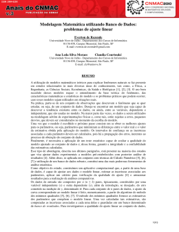
Diodes
1
Característica corrente-tensão do diodo ideal
Figure 3.1 The ideal diode: (a) diode circuit symbol; (b) i–v characteristic; (c) equivalent circuit in the
reverse direction; (d) equivalent circuit in the forward direction.
Copyright © 2004 by Oxford University Press, Inc.
2
Polarização direta e reversa dos diodos
Figure 3.2 The two modes of operation of ideal diodes and the use of an external circuit to limit the
forward current (a) and the reverse voltage (b).
Copyright © 2004 by Oxford University Press, Inc.
3
O retificador de meia onda
Figure 3.3 (a) Rectifier circuit. (b) Input waveform. (c) Equivalent circuit when vI ≥ 0. (d) Equivalent circuit
when vI — 0. (e) Output waveform.
Copyright © 2004 by Oxford University Press, Inc.
4
O retificador de meia onda
Copyright © 2004 by Oxford University Press, Inc.
5
Exercício 3.1
Esboçe a caracteristica de transferência do retificador de meia onda
Figure E3.1
Copyright © 2004 by Oxford University Press, Inc.
6
Exercício 3.2
Esboce a forma de onda da tensão no diodo.
Figure E3.2
Copyright © 2004 by Oxford University Press, Inc.
7
Carregador de Baterias
No circuito abaixo, de um carregador de baterias de 12 V, a tensão vS é
uma senoide de 24 V de amplitude.
1.
2.
3.
Determine a fração de um ciclo durante a qual o diodo conduz.
Determine o valor de pico da corrente no diodo.
Determine a tensão de pico inverso no diodo.
Figure 3.4 Circuit and waveforms for Example 3.1.
Copyright © 2004 by Oxford University Press, Inc.
8
Lócica com diodos
Determine a tabela verdade para cada um dos circuitos abaixo.
0 V corresponde a nível lógico zero e 5 V corresponde a nível lógico 1.
Figure 3.5 Diode logic gates: (a) OR gate; (b) AND gate (in a positive-logic system).
Copyright © 2004 by Oxford University Press, Inc.
9
Exemplo 3.2.
Supondo os diodos ideais, determine os valores de I e V.
Figure 3.6 Circuits for Example 3.2.
Copyright © 2004 by Oxford University Press, Inc.
10
Exercício 3.4 – Determine os valores de I e V.
Figure E3.4
Copyright © 2004 by Oxford University Press, Inc.
11
Exercício 3.4 – Determine os valores de I e V.
Copyright © 2004 by Oxford University Press, Inc.
12
Exercício 3.5
A figura mostra o circuito de um voltímetro C.A. Ele utiliza um medidor de
bobina móvel cujo fundo de escala corresponde a uma corrente igual a 1 mA.
O medidor tem uma resistência igual a 50 Ω. Determine o valor de R de modo
que o medidor indique o fundo de escala para uma senoide de entrada com
20 V pico a pico.
Figure E3.5
Copyright © 2004 by Oxford University Press, Inc.
13
Característica corrente – tensão de um diodo real
Figure 3.7 The i–v characteristic of a silicon junction diode.
Copyright © 2004 by Oxford University Press, Inc.
14
Característica corrente – tensão de um diodo real
IS – corrente de saturação
i = I S (e
v
nVT
− 1)
Figure 3.8 The diode i–v relationship with some scales expanded and others compressed in order to
reveal details.
Copyright © 2004 by Oxford University Press, Inc.
15
Equação do diodo
i = I S (e
v
nVT
− 1)
IS – corrente de saturação ou corrente de escala
• É da ordem de 10-15 A para pequenos diodos de sinais.
• É diretamente proporcional à área da seção transversal do diodo,
ou seja, diretamente proporcional à capacidade de corrente do diodo.
• Dobra de valor a cada aumento de 5 oC na temperatura.
Copyright © 2004 by Oxford University Press, Inc.
16
Equação do diodo
i = I S (e
kT
VT =
q
v
nVT
− 1)
Tensão térmica ≈ 25 mV a 20 oC
K – constante de Boltzmann = 1,38 x 10-23 joules/kelvin.
T = temperatura absoluta em graus kelvins = T(oC) + 273.
Q = carga do elétron = 1,60 x 10-19 C
n - constante do processo de fabricação.
n = 1 – diodos em circuitos integrados.
n = 2 – diodos discretos.
Copyright © 2004 by Oxford University Press, Inc.
17
Sejam (I1 ,V1) e (I2 ,V2) dois pontos da característica do diodo, na
região de polarização direta, então:
I1 = I S e
I2 = IS e
V1
nVT
V2
nVT
I2
I2
V2 − V1 = nVT ln
= 2,3VT log
I1
I1
Copyright © 2004 by Oxford University Press, Inc.
18
Variação da característica corrente – tensão do diodo com a temperatura
Figure 3.9 Illustrating the temperature dependence of the diode forward characteristic. At a constant
current, the voltage drop decreases by approximately 2 mV for every 1°C increase in temperature.
Copyright © 2004 by Oxford University Press, Inc.
19
Região de polarização reversa do diodo
i = I S (e
v
nVT
− 1)
Em polarização reversa, v é negativo, e:
i ≈ −I S
A corrente reversa de diodos é na verdade muito maior que IS, devido a
correntes parasitas que circulam externamente ao diodo.
A corrente reversa total dobra de valor para cada 10 oC de aumento da
temperatura.
Copyright © 2004 by Oxford University Press, Inc.
20
Exercício 3.9
Se V é igual a 1V a 20 oC, determine o valor de V a 40 oC e a 0 oC.
Figure E3.9
Copyright © 2004 by Oxford University Press, Inc.
21
Modelos para o diodo
Modelo exponencial
ID = ISe
VD
nVT
V DD − V D
ID =
R
Figure 3.10 A simple circuit used to illustrate the analysis of circuits in which the diode is forward
conducting.
Copyright © 2004 by Oxford University Press, Inc.
22
Modelo exponencial
Figure 3.11 Graphical analysis of the circuit in Fig. 3.10 using the exponential diode model.
Copyright © 2004 by Oxford University Press, Inc.
23
Análise Interativa
Exemplo 3.4
Determine a corrente ID e a tensão no diodo VD para o circuito da figura com
VDD = 5V e R = 1KΩ. Assuma que o diodo tem uma corrente de 1 mA com
uma tensão de 0,7 V e que sua tensão cai de 0,1 V para cada década de
variação de corrente.
Copyright © 2004 by Oxford University Press, Inc.
24
Modelo linear por partes
VD0 = 0,65 V
rD = 20Ω
Figure 3.12 Approximating the diode forward characteristic with two straight lines: the piecewise-linear
model.
Copyright © 2004 by Oxford University Press, Inc.
25
Modelo linear por partes
Figure 3.13 Piecewise-linear model of the diode forward characteristic and its equivalent circuit
representation.
Copyright © 2004 by Oxford University Press, Inc.
26
Exemplo 3.5
Determine a corrente ID e a tensão no diodo VD para o circuito da figura com
VDD = 5V e R = 1KΩ.
VD0 = 0,65 V
rD = 20Ω
Figure 3.14 The circuit of Fig. 3.10 with the diode replaced with its piecewise-linear model of Fig. 3.13.
Copyright © 2004 by Oxford University Press, Inc.
27
Modelo tensão constante
Figure 3.15 Development of the constant-voltage-drop model of the diode forward characteristics. A
vertical straight line (B) is used to approximate the fast-rising exponential. Observe that this simple model
predicts VD to within ±0.1 V over the current range of 0.1 mA to 10 mA.
Copyright © 2004 by Oxford University Press, Inc.
28
Modelo tensão constante
Figure 3.16 The constant-voltage-drop model of the diode forward characteristics and its equivalent-circuit
representation.
Copyright © 2004 by Oxford University Press, Inc.
29
Execício 3.12
Projete o circuito para fornecer uma tensão de saída igual a 2,4 V. Assuma que o diodo
tem uma corrente de 1 mA com uma tensão de 0,7 V e que sua tensão cai de 0,1 V para
cada década de variação de corrente.
Figure E3.12
Copyright © 2004 by Oxford University Press, Inc.
30
Modelo de pequenos sinais
ID = ISe
VD
nVT
Figure 3.17 Development of the diode small-signal model. Note that the numerical values shown are for
a diode with n = 2.
Copyright © 2004 by Oxford University Press, Inc.
31
Modelo de pequenos sinais
ID = ISe
VD
nVT
- corrente de polarização do diodo
v D (t ) = V D + v d (t )
i D (t ) = I S e
i D (t ) = I S e
(V D + v d )
nVT
VD
nVT
i D (t ) = I D e
e x ≈ 1 + x para x → 0
rd =
nVT
ID
e
vd
nVT
vd
nVT
i D (t ) ≈ I D (1 +
vd
)
nVT
Para:
vd
<< 1
nVT
resistência incremental do diodo
Copyright © 2004 by Oxford University Press, Inc.
32
Exemplo 3.6
A fonte V+ tem um valor médio igual a 10 V e um sinal sinal senoidal superposto
de 1V de amplitude e frequência igual a 60Hz. Calcule a tensão contínua nos
terminais do diodo e a amplitude da senoide que aparece em seus terminais. O
diodo apresenta uma queda de tensão de 0,7V em 1 mA e n = 2. R = 10 KΩ.
Figure 3.18 (a) Circuit for Example 3.6. (b) Circuit for calculating the dc operating point. (c) Small-signal
equivalent circuit.
Copyright © 2004 by Oxford University Press, Inc.
33
Exemplo 3.7
Três diodos são utilizados para fornecer uma tensão constante de 2,1 V.
Calcule a variação da tensão de saída causada por:
1.
2.
Um variação de ± 10% na tensão da fonte de alimentação.
Conexão de uma carga de 1KΩ.
Assuma n = 2.
Figure 3.19 Circuit for Example 3.7.
Copyright © 2004 by Oxford University Press, Inc.
34
O Diodo Zener
Figure 3.20 Circuit symbol for a zener diode.
Copyright © 2004 by Oxford University Press, Inc.
35
Característica i – v do diodo
VZ = VZ 0 + rz I Z
Figure 3.21 The diode i–v characteristic with the breakdown region shown in some detail.
Copyright © 2004 by Oxford University Press, Inc.
36
Modelo do diodo Zener
VZ = VZ 0 + rz I Z
Figure 3.22 Model for the zener diode.
Copyright © 2004 by Oxford University Press, Inc.
37
Exemplo 3.8
O diodo Zener da figura tem VZ = 6,8 V em IZ = 5 mA, rz = 20 Ω e IZK = 0,2 mA.
A fonte V+ é igual a 10 V e pode variar de ±1 V.
1.
Determine VO sem carga e V+ nominal.
2.
Determine a variação de VO devido a uma
variação de V+ de ±1 V.
3.
Determine a variação de VO resultante da
colocação de uma carga que solicita 1 mA.
4.
Determine o valor de VO quando RL = 2 KΩ.
5.
Determine o valor de VO quando RL = 0,5 KΩ.
Figure 3.23 (a) Circuit for Example 3.8. (b) The circuit with the zener diode replaced with its equivalent
circuit model.
Copyright © 2004 by Oxford University Press, Inc.
38
Solução
VZ = 6,8 V em IZ = 5 mA.
rz = 20 Ω
IZK = 0,2 mA
V+ =10 V ± 1 V.
Copyright © 2004 by Oxford University Press, Inc.
39
Circuitos Retificadores
Figure 3.24 Block diagram of a dc power supply.
Copyright © 2004 by Oxford University Press, Inc.
40
Retificador de meia onda
Figure 3.25 (a) Half-wave rectifier. (b) Equivalent circuit of the half-wave rectifier with the diode replaced
with its battery-plus-resistance model. (c) Transfer characteristic of the rectifier circuit. (d) Input and output
waveforms, assuming that rD <<R.
Copyright © 2004 by Oxford University Press, Inc.
41
Retificador de onda completa
Figure 3.26 Full-wave rectifier utilizing a transformer with a center-tapped secondary winding: (a) circuit;
(b) transfer characteristic assuming a constant-voltage-drop model for the diodes; (c) input and output
waveforms.
Copyright © 2004 by Oxford University Press, Inc.
42
Retificador em Ponte
Figure 3.27 The bridge rectifier: (a) circuit; (b) input and output waveforms.
Copyright © 2004 by Oxford University Press, Inc.
43
Retificador com filtro a capacitor
Figure 3.28 (a) A simple circuit used to illustrate the effect of a filter capacitor. (b) Input and output
waveforms assuming an ideal diode. Note that the circuit provides a dc voltage equal to the peak of the
input sine wave. The circuit is therefore known as a peak rectifier or a peak detector.
Copyright © 2004 by Oxford University Press, Inc.
44
Retificador de meia onda com filtro a capacitor
IL =
Vp
R
t
vo (t ) = V p e RC
−
I
Vr = L
fC
T
V p − Vr = V p e RC
−
Figure 3.29 Voltage and current waveforms in the peak rectifier circuit with CR @ T. The diode is assumed
ideal.
Copyright © 2004 by Oxford University Press, Inc.
45
Retificador de meia onda com filtro a capacitor
1
cos( wΔt ) ≈ 1 − ( wΔt ) 2
2
V p cos( wΔt ) = V p − Vr
wΔt =
2Vr
Vp
Intervalo de condução do diodo
Qcar = iCav Δt = Qdesc = CVr
i Dav = I L (1 + π
i Dmáx = I L (1 + 2π
iCav = i Dav − I L
2V p
Vr
)
2V p
Vr
Corrente média no diodo
) Corrente máxima no diodo
Copyright © 2004 by Oxford University Press, Inc.
46
Retificador de onda completa com filtro a capacitor
Vr =
Vp
2 fCR
i Dav = I L (1 + π
Vp
2Vr
)
i Dmáx = I L (1 + 2π
Vp
2Vr
)
Figure 3.30 Waveforms in the full-wave peak rectifier.
Copyright © 2004 by Oxford University Press, Inc.
47
Retificador de meia onda de precisão – O super diodo
Figure 3.31 The “superdiode” precision half-wave rectifier and its almost-ideal transfer characteristic. Note
that when vI > 0 and the diode conducts, the op amp supplies the load current, and the source is
conveniently buffered, an added advantage. Not shown are the op-amp power supplies.
Copyright © 2004 by Oxford University Press, Inc.
48
Circuitos limitadores
Figure 3.32 General transfer characteristic for a limiter circuit.
Copyright © 2004 by Oxford University Press, Inc.
49
Passando um sinal senoidal por um circuito limitador
Figure 3.33 Applying a sine wave to a limiter can result in clipping off its two peaks.
Copyright © 2004 by Oxford University Press, Inc.
50
Circuitos limitadores suaves
Figure 3.34 Soft limiting.
Copyright © 2004 by Oxford University Press, Inc.
51
Circuitos limitadores básicos
Copyright © 2004 by Oxford University Press, Inc.
Figure 3.35 A variety of basic limiting circuits.
52
Exercício 3.27
Supondo os diodos ideais, descreva a característica de transferência
do circuito.
Figure E3.27
Copyright © 2004 by Oxford University Press, Inc.
53
Circuito restaurador de nível C.C.
Figure 3.36 The clamped capacitor or dc restorer with a square-wave input and no load.
Copyright © 2004 by Oxford University Press, Inc.
54
Circuito restaurador de nível C.C. com carga resistiva
Figure 3.37 The clamped capacitor with a load resistance R.
Copyright © 2004 by Oxford University Press, Inc.
55
O dobrador de tensão
Figure 3.38 Voltage doubler: (a) circuit; (b) waveform of the voltage across D1.
Copyright © 2004 by Oxford University Press, Inc.
56
Princípio de operação dos diodos
Figure 3.39 Simplified physical structure of the junction diode. (Actual geometries are given in Appendix A.)
Copyright © 2004 by Oxford University Press, Inc.
57
Ligações covalentes
Figure 3.40 Two-dimensional representation of the silicon crystal. The circles represent the inner core of
silicon atoms, with +4 indicating its positive charge of +4q, which is neutralized by the charge of the four
valence electrons. Observe how the covalent bonds are formed by sharing of the valence electrons. At 0 K,
all bonds are intact and no free electrons are available for current conduction.
Copyright © 2004 by Oxford University Press, Inc.
58
Ionização térmica
n – concentração de elétrons
p – concentração de buracos
ni – concentração intrínsica
n = p = ni
Figure 3.41 At room temperature, some of the covalent bonds are broken by thermal ionization. Each
broken bond gives rise to a free electron and a hole, both of which become available for current
conduction.
Copyright © 2004 by Oxford University Press, Inc.
59
Concentração intrínseca
B = 5,4 x 1031 para o silício
ni2
=
E
− G
BT 3e kT
EG = 1,12 eV para o silício
k = 8,62 x 10-5 eV/K
Na temperatura ambiente, ni = 1,5 x 1010 portadores/cm3
Um cristal de silício tem 5 x 1022 átomos por cm3
Copyright © 2004 by Oxford University Press, Inc.
60
Corrente de Difusão
Dp = 12 cm2/s – constante de difusão de buracos
Dn = 34 cm2/s – constante de difusão de elétrons
J p = −qD p
dp
dx
Jp – densidade de corrente de buracos - A/cm2
Jn – densidade de corrente de elétrons - A/cm2
J n = qDn
dn
dx
Figure 3.42 A bar of intrinsic silicon (a) in which the hole concentration profile shown in (b) has been
created along the x-axis by some unspecified mechanism.
Copyright © 2004 by Oxford University Press, Inc.
61
v drift = μ p E
Corrente de Drift
-
J p − drift = qpμ p E
+
-
J n − drift = qnμ n E
+
-
+
-
+
-
+
+
E
L
J drift = q( nμ n + pμ p ) E
-
µp = 480 cm2/V.s – mobilidade dos buracos
µn = 1350 cm2/V.s – mobilidade dos elétrons
Copyright © 2004 by Oxford University Press, Inc.
V
i
= q ( nμ n + pμ p )
A
L
ρ=
1
q ( pμ p + n μ n )
Relação de Einstein
Dn
μn
=
Dp
μp
= VT
62
Semicondutores Dopados
Material tipo n: dopado com substâncias doadoras. Ex: fósforo
nn0 ≅ N D
nn0 p n0 = ni2
ni2
p n0 =
ND
Figure 3.43 A silicon crystal doped by a pentavalent element. Each dopant atom donates a free electron
and is thus called a donor. The doped semiconductor becomes n type.
Copyright © 2004 by Oxford University Press, Inc.
63
Semicondutores Dopados
Material tipo p: dopado com substâncias aceitadoras. Ex: boro
p p0 ≈ N A
nn0 p n0 = ni2
ni2
nn0 =
NA
Figure 3.44 A silicon crystal doped with a trivalent impurity. Each dopant atom gives rise to a hole, and the
semiconductor becomes p type.
Copyright © 2004 by Oxford University Press, Inc.
64
A junção pn em circuito aberto
ID = IS
qx p AN A = qx n AN D
xn
NA
=
xp ND
V0 = VT ln(
Wdep = x n + x p =
2ε S
q
⎛ 1
1
⎜⎜
+
⎝ N A ND
N AND
ni2
)
⎞
⎟⎟V0
⎠
Figure 3.45 (a) The pn junction with no applied voltage (open-circuited terminals). (b) The potential
distribution along an axis perpendicular to the junction.
Copyright © 2004 by Oxford University Press, Inc.
65
A junção pn polarizada reversamente
Figure 3.46 The pn junction excited by a constant-current source I in the reverse direction. To avoid
breakdown, I is kept smaller than IS. Note that the depletion layer widens and the barrier voltage increases
by VR volts, which appears between the terminals as a reverse voltage.
Copyright © 2004 by Oxford University Press, Inc.
66
Capacitância de transição
Cj =
dq j
dV R
V R =VQ
Figure 3.47 The charge stored on either side of the depletion layer as a function of the reverse voltage VR.
Copyright © 2004 by Oxford University Press, Inc.
67
A junção pn polarizada diretamente
Figure 3.49 The pn junction excited by a constant-current source supplying a current I in the forward
direction. The depletion layer narrows and the barrier voltage decreases by V volts, which appears as an
external voltage in the forward direction.
Copyright © 2004 by Oxford University Press, Inc.
68
Distribuição de portadores minoritários
Figure 3.50 Minority-carrier distribution in a forward-biased pn junction. It is assumed that the p region is
more heavily doped than the n region; NA @ ND.
Copyright © 2004 by Oxford University Press, Inc.
69
Problema 3.2
Supondo o diodo ideal, calcule os valores de I e V.
Figure P3.2
Copyright © 2004 by Oxford University Press, Inc.
70
Problema 3.3
Supondo o diodo ideal, calcule os valores de I e V.
Figure P3.3
Copyright © 2004 by Oxford University Press, Inc.
71
Problema 3.4
Em cada circuito, vI é uma senoide de 10 V de amplitude e frequência de 1 kHz.
Esboce a forma de onda de vo supondo os diodos ideais.
Figure P3.4 (Continued)
Copyright © 2004 by Oxford University Press, Inc.
72
Problema 3.4
Em cada circuito, vI é uma senoide de 10 V de amplitude e frequência de 1 kHz.
Esboce a forma de onda de vo supondo os diodos ideais.
Figure P3.4 (Continued)
Copyright © 2004 by Oxford University Press, Inc.
73
Problema 3.5
Figure P3.5
Copyright © 2004 by Oxford University Press, Inc.
74
Problema 3.6
Figure P3.6
Copyright © 2004 by Oxford University Press, Inc.
75
Problema 3.9
Supondo os diodos ideais, determine as correntes e tensões indicadas.
Figure P3.9
Copyright © 2004 by Oxford University Press, Inc.
76
Problema 3.10
Assumindo os diodos ideais, utilize o teorema de Thevenin para simplificar os
circuitos e então determine os valores das tensões e correntes indicadas.
Figure P3.10
Copyright © 2004 by Oxford University Press, Inc.
77
Problema 3.16
Figure P3.16
Copyright © 2004 by Oxford University Press, Inc.
78
Problema 3.23
Figure P3.23
Copyright © 2004 by Oxford University Press, Inc.
79
Problema 3.25
Na figura, ambos diodos tem n=1, mas D1 tem 10 vezes a área de junção de
D2. Qual o valor de V ? Qual deve ser o valor de I2 para obter V = 50 mV.
Figure P3.25
Copyright © 2004 by Oxford University Press, Inc.
80
Problema 3.26
Os diodos são idênticos conduzindo 10 mA com 0,7 V e 100 mA em 0,8 V.
Determine o valor de R para V = 80 mV.
Figure P3.26
Copyright © 2004 by Oxford University Press, Inc.
81
Problema 3.28
Figure P3.28
Copyright © 2004 by Oxford University Press, Inc.
82
Problema 3.54
Figure P3.54
Copyright © 2004 by Oxford University Press, Inc.
83
Problema 3.56
Figure P3.56
Copyright © 2004 by Oxford University Press, Inc.
84
Problema 3.57
Figure P3.57
Copyright © 2004 by Oxford University Press, Inc.
85
Problema 3.58
Figure P3.58
Copyright © 2004 by Oxford University Press, Inc.
86
Problema 3.59
Figure P3.59
Copyright © 2004 by Oxford University Press, Inc.
87
Problema 3.63
Figure P3.63
Copyright © 2004 by Oxford University Press, Inc.
88
Problema 3.82
Figure P3.82
Copyright © 2004 by Oxford University Press, Inc.
89
Problema 3.91
Figure P3.91
Copyright © 2004 by Oxford University Press, Inc.
90
Problema 3.92
Figure P3.92
Copyright © 2004 by Oxford University Press, Inc.
91
Problema 3.93
Figure P3.93
Copyright © 2004 by Oxford University Press, Inc.
92
Problema 3.97
Figure P3.97
Copyright © 2004 by Oxford University Press, Inc.
93
Problema 3.98
Figure P3.98
Copyright © 2004 by Oxford University Press, Inc.
94
Problema 3.102
Figure P3.102
Copyright © 2004 by Oxford University Press, Inc.
95
Problema 3.103
Figure P3.103
Copyright © 2004 by Oxford University Press, Inc.
96
Problema 3.105
Figure P3.105
Copyright © 2004 by Oxford University Press, Inc.
97
Problema 3.108
Figure P3.108
Copyright © 2004 by Oxford University Press, Inc.
98