Optimising land use
and water allocation
in intercropping
systems1
Euro Roberto Detomini2
Margarida Garcia de Figueiredo3
Abstract – The main purpose of this study is to identify the optimum allocation of limited amount of
land and irrigation water across a number of alternative farm enterprises, maximising the whole-farm
profitability by considering present relative prices, changes in river water availability, irrigation system efficiency and a highly variable climate. It was developed an optimisation model by using linear
programming language to maximise the whole-farm profit of farm located in Wee Waa (NSW, Australia), for three different scenarios (dry, average and wet years) over two seasons. The whole-farm
profit is highly sensitive to climate variability and also to prices and yields variability, especially in
relation to cotton.
Keywords: Crop rotation, linear programming, profit maximization.
Otimização do uso da terra e da alocação
de água em sistemas de rotação de culturas
Resumo – O principal objetivo deste estudo de caso é identificar a alocação ótima de recursos,
especificamente água para irrigação e terra, entre alternativas de atividades agrícolas, visando maximizar o lucro da propriedade, considerando preços relativos, mudanças na disponibilidade de água,
eficiência do sistema de irrigação e alta variabilidade climática. Foi desenvolvido um modelo de
programação linear, com o objetivo de maximizar o lucro das atividades agrícolas de uma propriedade localizada em Wee Waa (NSW, Austrália), considerando três cenários (seco, médio e úmido,
conforme a variabilidade do regime de chuvas) ao longo de 2 anos. O lucro total da propriedade
mostrou-se altamente sensível à variabilidade climática, bem como às variações nos preços e ao
rendimento produtivo das culturas, especialmente com relação ao algodão.
Palavras-chave: rotação de culturas, programação linear, maximização de lucro.
1
Original recebido em 24/10/2011 e aprovado em 11/11/2011.
2
Agronomist, Ph.D. in Irrigation and Drainage. E-mail: [email protected] (corresponding author)
3
Agronomist, Ph.D. in Economy. E-mail: [email protected]
Ano XXI – No 1 – Jan./Fev./Mar. 2012
92
Introduction
In Australia, cotton farmers confront the
challenges of drought, increased climate variability and poor business profitability, driven by
low yields, low prices and increased costs. Despite profit from cotton remains better than most
broad acre rainfed crops, high yielding cereals
grown on limited water are providing higher
profitability per mega litre of water. This is the
reason why Australian growers are interested in
identifying opportunities that maximise returns
per mega litre by considering the crop rotations
between cotton and cereal, instead of planting
cotton back to back.
Because of that and considering the increased focus on more economic and environmental sustainable farm systems, there is an
increased interest in building models to improve
the whole-farm profitability in a sustainable way.
These whole-farm models are able to predict the
impacts of different scenarios not only in terms
of climate variability, but also prices, yields and
costs variability. Also, whole-farm models can
be complemented by simple analysis or specific
economic models such as that ones of Engindeniz and Tuzel (2006) or Beltrame et al. (2007),
respectively. As a crop rotation system has a
major impact on environment sustainability and
productivity increase due to improve yields, soil
characteristics, diseases control, etc., it addresses
a more economic and environmental sustainable production system. Thus, the whole-farm
models which include crop production must
somehow include crop rotation as an important
component (DETLEFSEN; JENSEN, 2007).
Optimisation models are developed to
give farmers support in decision making related
to what to plant, where in the farm and when,
to maximise the whole-farm profitability by identifying the optimum resources allocation across
a number of alternative farm enterprises in crop/
grazing rotation systems. Optimisation models can be developed using linear programming
(LP) language. LP is an upgrade of a linear equation system’s resolution technique through a sequence of matrixes inversion, with the advantage
93
of including an additional linear equation which
represents an objective to be achieved in terms of
maximisation or minimisation (CHVÁTAL, 1983).
This work was done adopting a study case
of an Australian cotton/grain farming system,
specifically from Wee Waa, New South Wales,
but the idea can be extrapolated elsewhere.
The goal is to present an optimisation methodology based on operational research, indicating
the best trade-off between land and water use in
this agricultural system by analysing the best net
return of the whole agricultural activity throughout the years of crop rotation in a farm scale.
Methodology
The currently most used algorithm in linear
programming (LP) softwares is the Simplex Method which was developed during the Second War
in 1947 by a Northern American scientist staff,
and has been published afterwards. However,
breakthrough in terms of correlated algorithms
efficiency only could be observed in the 1980’s
through developed studies (KAMARKAR, 1984).
Nowadays, LP is broadly used around the world
and can be applied for different objectives such
as maximise profits, efficiency, social welfare,
etc.; or minimise costs, time, losses, etc.
A LP model can be summarised as:
n
MaxZ = Σ cj Xj
j=1
(1)
Subject to:
n
Σ a X ≤ bi , i = 1, 2, …, m
j=1 ij j
(2)
Xj ≥ 0, j = 1, 2, …, n
(3)
in which
cj represents the j activity’s gross margin.
Xj represents the j activity’s level.
aij represents the each input exigency by
each activity.
bj represents the each input availability.
Ano XXI – No 1 – Jan./Fev./Mar. 2012
Equation 1 represents the objective function.
Equation 2 represents the functional
constrains.
Equation 3 represents the non-negativity
constrains.
The variables in a LP model cannot assume
negative values, although these can be expressed
as a difference between two positive variables. All
involved equations must be linear, which means,
all coefficients have a constant behaviour. The restrictions expressed as unequal equations allow
that the whole use of resources be not mandatory
and the explored level of any activity can be more
than or equal zero. The LP models allow a much
wider range of response by farmers in their choice
of outputs and inputs than the limited number of
alternatives presented in other methodologies, for
example in budgeting studies. In addition, LP is
a powerful optimising technique in that it selects
the combination of enterprises that will maximise
profits from a specified set of enterprises subject to
specified resource constraints set. An added advantage of LP is that they provide dual prices information indicating the change in profit when additional
units of a limited resource were made available.
Thus, specifically in this case study it was developed an optimisation model, by using LP language,
to maximise the whole-farm profit of a 1,348 ha
farm located in Wee Waa (NSW). The necessary
information to be included as the inputs in the optimisation model was collected from an interview
with the farm manager. Moreover, it was collected
information from QL-DPI&F and NSW-DPI&F cotton-irrigation researchers. As the whole-farm profit
can be highly affected by the climate variability, the
analysis was developed for three different scenarios: typically dry, average and wet years.
In addition to changes in climate, the irrigation system efficiency variability and the prices
and crop yields variability may have significant
effects on the farm business profitability. Thus, it
was performed a sensitivity analysis on the variability of irrigation system efficiency, prices and
yields to evaluate their influence on the wholefarm maximum return. The irrigation system ef-
ficiency was varied from 40% to 90%; prices
and yields, for each of the crops, were individually varied by ±10%, ±20%, ±30% and ±40%.
The central purpose of this work is to show how
the whole-farm profitability can be improved
through the optimum allocation of land and water across a number of alternative farm enterprises, face on high variability of prices, yields, costs
and climate condition.
The Crop Rotation
Optimisation Model
The optimisation model was developed by
considering five different enterprises as the objective function variables, i.e. irrigated cotton, irrigated maize, rainfed wheat, irrigated wheat (with
1 irrigation) and irrigated wheat (with 2 irrigations). In addition, it was considered two different
seasons, where the first one goes from May of
year 1 to February of year 2 and the second one
goes from October of year 2 to April of year 3.
Variable Description:
1) Five Crops: (i = 1, 2, 3, 4, 5); where
Crop 1 = Irrigated cotton; Crop 2 = Irrigated maize; Crop 3 = Rainfed wheat;
Crop 4 = Irrigated wheat (1 irrigation);
Crop 5 = Irrigated wheat (2 irrigations).
2) Two Seasons: ( j = 1, 2): Season 1 = May
year 1 – February year 2; Season 2 =
October year 2 – April year 3.
The objective function is a linear equation
which can represent different objectives to be
achieved such as maximise profits, efficiency, social welfare, etc.; or minimise costs, time, losses,
etc. Specifically in this case study the objective
is to maximise the whole-farm profit so that the
equation coefficients represent the gross margin
($/ha) associated to each enterprise to be implemented. The variables of interest are the area (ha)
to be cultivated with each activity. Other important feature of linear programming models is related to the constraints set represented by unequal
equations that allow the whole use of resources
be not mandatory. In this case study the func-
Ano XXI – No 1 – Jan./Fev./Mar. 2012
94
tional constraints are related to water and land
availability over each season, which means, the
maximum area to be cultivated in each season
must be smaller than the total available area and
the maximum water use in each season must not
be more than the available water from rain, soil
moisture and irrigation system.
Objective Function:
5
2
Max Σ Σ Gij X ij
i=1 j=1
i = crop
j = season
G = gross margin ($/ha)
Subjected to the following constraints:
1) Land restriction:
5
ΣX ≤ A
i=1 i1
Season 2:
ΣX ≤ A
i=1 i2
5
A = Area
2) Area balance each season:
5
Season 1:
Σ X – TA = 0
i=1 i1
Season 2:
Σ X – TA = 0
i=1 i2
5
TA = Total area
3) Water restriction:
Season 1:
Season 2:
5
ΣW X ≤ W
i=1 i1 i1
5
Σ Wi2 X i2 ≤ W
i=1
Wi1 = Water consumed per crop i, during
the cycle, on season 1; Wi2 = Water consumed
per crop i, during the cycle, on season 2; W =
Total water availability during each season.
95
X ij ≥ 0
i = 1, 2, 3, 4, 5
j = 1, 2
After developing the optimisation model the next step should be apply it based on
empirical data set in order to verify its practical
applicability. Thus, the methodology was empirically tested based on a data set collected from
an interview with the studied farm’s manager as
showed in the next section.
Data set considered
for the case study
X = area (ha)
Season 1:
4) Non-negativity restrictions:
The case study was developed based on an
interview with the farm manager of a grain-cotton irrigation farm system located in Wee Waa,
NSW. In addition to the farm manager, it was collected information from QLD-DPI&F and NSWDPI&F cotton-irrigation expertises. The studied
farm business has a total area of 1,348 ha with
a soil type of 250 mm under full Plant Available
Water Capacity (PAWC). The analysis was developed under three different scenarios: Table 1)
Dry year: low water availability from soil + rainfall and irrigation; Table 2) Average year: plenty of water availability; Table 3) Wet year: high
water availability. Two seasons were considered
into the model: (1) Season 1: From May to February (sow wheat in May or maize in August) and
(2) Season 2: From October to April (sow cotton
in October). It was assumed a fallow efficiency
of 30%; and 125 mm 50% PAWC over the dry
year scenario, 188 mm 75% PAWC over the average year scenario and 250 mm 100% PAWC
over the wet year scenario.
The sources of irrigation water were river
or bore. Therefore, the costs of irrigation were
different for the different scenarios i.e. the dryer
the season, the lower the river allocation and, as
a consequence, the higher the allocation cost.
The three tables below summarise the variables
and assumed values used to calculate gross mar-
Ano XXI – No 1 – Jan./Fev./Mar. 2012
Table 1. Inputs to the optimisation model: dry year.(1)
Variables
1) Price ($/t)
2) Yield (bales/ha or t/ha)
3) Variable cost ($/ha)
(2)
4) Water cost ($/ML water)
5) Water delivered to the crop
(ML/ha.year)
Irrigated
cotton
Irrigated
maize
Rainfed
wheat
Wheat 1
irrigation
Wheat 2
irrigations
$458
$250
$200
$200
$200
9
10
2
5
7
$2,100
$749
$465
$550
$590
$66.67
$66.67
–
$66.67
$66.67
7
7
–
1.5
3
6) Irrigation cost ($/ha)
$467
$467
$0
$100
$200
7) Gross margin ($/ha)
$1,457
$1,210
-$65
$337
$601
8) Gross margin ($/ML)
$208
$173
$0
$224
$200
(1)
Data collected from the farm manager.
(2)
Variable cost source = DPI (NSW) / Farm Enterprise Budget Series – Northern Zone/2005–2006.
Table 2. Inputs to the optimisation model: average year.(1)
Variables
1) Price ($/t)
2) Yield (bales/ha or t/ha)
3) Variable cost ($/ha)
(2)
4) Water cost ($/ML water)
Irrigated
cotton
Irrigated
maize
Rainfed
wheat
Wheat 1
irrigation
Wheat 2
irrigations
$458
$200
$200
$200
$200
3
6
8
$465
$550
$590
10
11.25
$2,100
$749
$46.42
$46.42
–
$46.42
$46.42
6
6
–
1.5
2.5
6) Irrigation cost ($/ha)
$278
$278
$0
$70
$116
7) Gross margin ($/ha)
$2,160
$1,190
$35
$604
$897
8) Gross margin ($/ML)
$360
$198
$0
$402
$359
5) Water delivered to the crop
(ML/ha.year)
(1)
Data collected from the farm manager.
(2)
Variable cost source = DPI (NSW) / Farm Enterprise Budget Series – Northern Zone/2005–2006.
Table 3. Inputs to the optimisation model: wet year.(1)
Variables
1) Price ($/t)
2) Yield (b/ha or t/ha)
3) Variable cost(2) ($/ha)
4) Water cost ($/ML water)
5) Water delivered to the crop
(ML/ha.year)
Irrigated
cotton
Irrigated
maize
Rainfed
wheat
Wheat 1
irrigation
Wheat 2
irrigations
$458
$180
$200
$200
$200
8.5
12.5
3.8
7.5
8.0
$2,100
$749
$465
$550
$590
$40
$40
–
$40
$40
4.5
4.5
–
1.25
2
6) Irrigation cost ($/ha)
$180
$180
$0
$50
$80
7) Gross margin ($/ha)
$1,584
$1,304
$295
$947
$921
8) Gross margin ($/ML)
$352
$290
$0
$757
$460
(1)
Data collected from the farm manager.
(2)
Variable cost source = DPI (NSW) / Farm Enterprise Budget Series – Northern Zone/2005–2006.
Ano XXI – No 1 – Jan./Fev./Mar. 2012
96
gins ($/ha; inputs in the Optimisation Model)
for each crop over dry, average and wet years,
respectively. The considered crops are irrigated
cotton, irrigated maize, rainfed wheat and wheat
with one and two irrigations.
Information about rainfall (mm) in Wee
Waa, over the considered periods (Seasons 1
and 2), was collected from SILO (JEFFREY et al.,
2001) to the last 100 years. The rainfall pattern
was considered different among the scenarios,
which means, across the 100 observations for
each season, the lower, the average and the higher values were associated to dry, average and wet
scenarios, respectively, as showed in Table 4.
According to the farm manager’s information, the
water availability to irrigation per season would
be considered in each scenario as: (i) Dry year:
2,000 ML (from Bore) + 1,000 ML (from River) =
3,000 ML; (ii) Average year: 2,000 ML (from
Bore) + 3,300 ML (from River) = 5,300 ML; and
(iii) Wet year: 2,000 ML (from Bore) + 5,000 ML
(from River) = 7,000 ML.
The total water availability (including both,
from irrigation and from soil + rainfall) considered per season, in each scenario, is described in
the Table 5 and Table 6, and the water allocation
cost was considered different among the three
scenarios, as showed in Table 7.
Table 4. Rainfall pattern (mm) in Wee Waa, NSW,
Australia.
Season 1
Season 2
Scenario
Rainfall from
May to February
Rainfall from
October to April
Dry year
355 mm
276 mm
Average year
473 mm
363 mm
Wet year
648 mm
512 mm
Source: Jeffrey et al. (2001).
Table 5. Total water availability over Season 1.
(II)
(I)
Season
(I + II)
Soil + rainfall
Total
Irrigation
(ML/ Season) (ML/ Season) (ML/ Season)
(1)
Dry
2,100 ML
3,114 ML
5,214 ML
Average
3,710 ML
4,448 ML
8,158 ML
Wet
4,900 ML
5,985 ML
10,885 ML
(1)
It was assumed an irrigation efficiency of 70% so that the irrigation water
availability was multiplied per 0.7.
Table 6. Total water availability over Season 2.
(II)
(I)
Season
(I + II)
Soil + rainfall
Total
Irrigation
(ML/ Season) (ML/ Season) (ML/ Season)
(1)
Results and discussion
Dry
2,100 ML
2,790 ML
4,890 ML
The optimum use of land across different
crop options, in order to maximise the wholefarm profit, over a two-year period, subject to
water constraints and taking in account the present relative prices for cotton, maize and wheat
is summarised in Table 8. In a typical dry year,
for the first season, the maximum profit was obtained from planting 652 ha of irrigated maize,
whereas for the second season the maximum
profit was obtained from planting 611 ha of irrigated cotton. The same interpretation can be
done for typically average and wet years. By
adopting such strategies, the whole-farm profits
were $ 1,679,209; $ 3,483,832 and $ 3,893,024
over dry, average and wet years, respectively.
Average
3,710 ML
4,004 ML
7,714 ML
Wet
4,900 ML
5,446 ML
10,346 ML
97
(1)
It was assumed an irrigation efficiency of 70% so that the irrigation water
availability was multiplied per 0.7.
Table 7. Water allocation cost(1).
Allocation
Average
cost
Dry
67% from Bore / 33% from River
$67/ML
Average
38% from Bore / 62% from River
$46/ML
Wet
29% from Bore / 71% from River
$40/ML
Season
(1)
River = $ 20/ML; Bore = $ 90/ML.
Ano XXI – No 1 – Jan./Fev./Mar. 2012
Table 8. Optimum crop allocation over seasons 1 and 2 for dry, average and wet years.
Scenario
Season 1
Season 2
Dry year
652 ha of irrigated maize
611 ha of irrigated cotton
Average year
473 ha of irrigated maize
990 ha to irrigated cotton
875 ha of wheat with 2 irrigations
Wet year
1,348 ha of irrigated maize
Once maize is priced internally in the Australian market, its price is highly affected by different climate conditions, being relatively low in
wet seasons and raising gradually from wet to dry
seasons. Alternatively, cotton and wheat prices
are not affected by climate conditions, where the
former is determined in the international market,
whereas the latter usually does not change due
to contracted prices. Despite maize being more
water exigent than wheat, throughout dry years
it is interesting to plant only maize in season 1
instead of doing wheat. As maize not only has
a higher yield but also has a higher price, in
comparison to wheat, maize gross margin is approximately twice as higher than that of wheat.
Consequently, to plant only maize is economically more interesting for typically erratic rain
years.
According to the farm manager’s information, the maize and wheat prices are roughly the
same if the scenario is considered average. However, the maize gross margin is still higher than
that of wheat in that case due to the higher maize
yield. In that context, there is reasonable water
availability for planting and the most appropriated strategy in terms of profit maximisation would
1,348 ha to irrigated cotton
be to plant a larger area of wheat, given that
its water consume is approximately 40% lower
than that for maize. It is important to consider
that throughout the average situation maize gross
margin is no longer twice as higher than that of
wheat, decreasing for 33% higher. By considering the wet scenario, despite maize price being
lower than wheat price, the maize gross margin
is still higher than that to wheat, in approximately
42%. Once in a typically wet year there is plenty
of available water, the economically most interesting strategy would be to plant only irrigated
maize during the first season instead of planting
irrigated wheat in a part of the area.
Other interesting information from a linear
programming resolution is the dual price, which
represents the objective function value variation
(whole-farm profit in this specific case) due to
a unitary variation in a binding constrain value.
Only binding constraints have a dual price value,
and for those nonbindings, the dual price is zero,
as summarised in Table 9. For example, for the
dry scenario, the land constraints were nonbinding, whereas the water constraints were binding
in both, seasons 1 and 2. In that case, if one extra
ML of water per hectare were made available,
Table 9. Dual price analysis to water and land restrictions.
Restrictions
Dry year
Average year
Wet year
Dual price ($)
Dual price ($)
Dual price ($)
Land season 1
0.00
408.66
1,304.00
Land season 2
0.00
0.00
1,584.00
Water season 1
151.25
97.66
0.00
Water season 2
182.13
276.92
0.00
Ano XXI – No 1 – Jan./Fev./Mar. 2012
98
the whole-farm profit could be increased in $151
and $182, over seasons 1 and 2, respectively. So,
these values are the maximum amount the farm
would be willing to pay for one additional ML of
water per hectare.
As over the average scenario there was
reasonable water availability for planting and
wheat is less exigent in water when compared
with cotton and maize, for the first season, when
the optimum strategy was to plant 65% of the
total area with wheat and 35% with maize, both
constraints (land and water) were binding. In this
case, if one extra hectare or one extra ML of water per hectare were made available, the wholefarm profit could be increased in $408 and $97,
respectively. For the second season, only the
water availability was a binding constraint and
if one extra ML of water per hectare were made
available, the farm profit could be increased in
$276. As cotton has a high water exigency over
its cycle, the optimum strategy was to plant 73%
of the total area with cotton so that the land
availability was not a binding constraint.
For the wet scenario, when there was
plenty of available water, only the land availability was a binding constraint for both seasons. If
one extra hectare were made available, the profit
could be increased in $ 1,304 and $ 1,584, over
the seasons 1 and 2, respectively. Changes in ir-
rigation system efficiency can have significant effects on the farm business viability so that it was
performed a sensitivity analysis on irrigation system efficiency to evaluate its influence on maximum farm profit. The irrigation system efficiency
was varied from 40% to 90%, by assuming 70%
as the most likely efficiency. Figure 1 shows the
maximum return (over a two-year period) variation for different irrigation system efficiency values over dry, average and wet years, through a
variation index around 70% efficiency (70% =
100). It can be observed that the maximum return is more sensitive to the irrigation system efficiency over dry years and it gets gradually less
sensitive from average to wet years. In a typically
dry year the production system is highly dependent of irrigation so that especially for the dry
scenario the whole-farm profit is highly sensitive
to the irrigation system efficiency.
Figure 2a shows a variation index of maximum farm profit for each change in price (or
yield) over the dry scenario, where values above
100 indicate higher profitability and values below 100 indicate lower profitability, in relation
to the most likely profitability (when considering the most likely price and the most likely
yield). Figure 2b and Figure 2c present similar
information for the average and wet scenarios,
respectively. Cotton has a high production cost,
a high price and a high gross margin ($/ha) when
Figure 1. Sensitivity of maximum return to changes in irrigation system efficiency during dry, average and wet seasons.
99
Ano XXI – No 1 – Jan./Fev./Mar. 2012
a
b
c
Figure 2. a) Sensitivity of maximum return to changes in prices (or yields) during dry years; b) Sensitivity of maximum return to changes in prices (or yields) during average years; and c) Sensitivity of maximum return to changes
in prices (or yields) during wet years.
compared with other crops so that it can contribute considerably to improve the whole-farm
profitability. Consequently, the maximum return
to be achieved is highly sensitive to variations in
cotton price (or yield). As cotton is priced externally, in the international market, and also is
highly exigent in water over its cycle, it addresses
a risky production system in relation to climate
and market variability. Economic sustainability
means to increase profitability and to decrease
the variability of profitability throughout the
time. From the economic point of view, the more
diversified a business is the less risky it is in terms
of profitability’s variability. If a problem with
Ano XXI – No 1 – Jan./Fev./Mar. 2012
100
some specific activity comes, for example a crop
disease, the whole-farm profitability is not highly
affected because there are other activities being
conducted at the same time. Moreover, when
adopting a crop rotation system, the whole-farm
profitability can be improved by deciding what
to plant, where in the farm and when, according
markets forces (present relative prices of crops)
and resources availability.
Summarising the results, in a typically dry
year, the maximum farm profitability was obtained with a combination of 65% of the farm
area to irrigated maize, during the first season,
and 45% to irrigated cotton, during the second
season. In average years, the optimum strategy
would be to plant 65% of the farm area with
wheat with 2 irrigations and 35% with irrigated
maize, during the first season, and 73% with irrigated cotton, during the second season. In a typically wet year, the optimum allocation would be
to plant 100% of the area with irrigated maize,
during the first season, and 100% with irrigated
cotton, during the second season. By adopting
such strategies, the maximum profits, over a
two-year period, were $1,679,209; $3,483,832
and $3,893,024 for dry, average and wet years,
respectively.
The scenarios evaluated here were considered realistic and the outcomes indicate that the
whole-farm profitability can be improved by adjusting the farm business strategy i.e. optimising
the land use among a number of alternative irrigated crop options, according to seasonal conditions and water availability to irrigation. As the
maximum return is highly sensitive to irrigation
system efficiency, especially during dry years, it
is important to work towards improve it. A suggestion would be changing from furrow irrigation
systems to pressurised ones, given that the latter
are usually more efficient. However, before making a decision it would be necessary to evaluate
the economic viability and also the associated
risks. Therefore, for future studies it would be
interesting to include similar evaluations to that
one developed by Qureshi et al. (2001), who
compared different irrigation technology systems
101
for farms located in north Queensland, in order
to identify the economic viability and the main
implications in terms of investment decision
when changing from furrow to pivot systems.
The results also indicate the need for a
more accurate study to better capture the dynamics and complexities of the studied farm in terms
of the optimal allocation of competing resources
i.e. water, land, finances, productivity and labour.
Additional interviews with some farm managers
to ask more specific information and also other
methodologies, such as non-linear programming
(GHAHRAMAN; SEPASKHAH, 2004), multi-objective optimisation techniques (FLORENTINO
et al., 2008), evolutionary algorithms, etc., could
be used for that purpose. Once the whole-farm
profit is highly sensitive to climate variability and
also to prices and yields variability, especially in
relation to cotton, it would be interesting for future studies to use stochastic procedures as done
by Ganji et al. (2006) to introduce risk analysis
into the model in relation to prices, yields and
climate variability, regardless of the pragmatic
separation of the conditions in wet, average or
dry years. Therefore, it is important to consider
that optimisation models can be used to identify
the optimum allocation of water and land use
in irrigated agriculture, though the analysis needs
to be complemented with an evaluation of business viability and cash flow. This is because of
the main input variable in the optimisation model is the gross margin ($/ha) of each farm activity,
which excludes the opportunity cost of money
(interest rate), and the fixed costs i.e. the value
of the land/improvements, buildings, machinery
and agricultural wares.
The best trade-off between water and
land use will carry to the preconised, necessary
and so mentioned sustainable irrigation. Therefore, as adequate knowledge already exists for
implementing strategies to achieve sustainable irrigation (OSTER; WICHELNS, 2003) and following the approach of Hellegers (2006), although
conciliating economic analysis in irrigation with
aspects of environment dynamics and people income distribution, being this essentially political,
Ano XXI – No 1 – Jan./Fev./Mar. 2012
the economic interpretation performs a crucial
role not only because of providing the basis of
decision support or understanding the gross margins and financial losses of agricultural systems,
but also in terms of the comprehension of the interactions of the mentioned elements, given that
incorporates criteria of water use and contributes
to promote social welfare, which is the final target of public policies (i.e., agricultural policies).
Conclusions
In a typically dry year, the maximum farm
profitability was obtained with a combination
of 65% of the farm area to irrigated maize, during the first season, and 45% to irrigated cotton,
during the second season. In average years, the
optimum strategy would be to plant 65% of the
farm area with wheat with two irrigations and
35% with irrigated maize, during the first season,
and 73% with irrigated cotton, during the second season. In a typically wet year, the optimum
allocation would be to plant 100% of the area
with irrigated maize, during the first season, and
100% with irrigated cotton, during the second
season.
DETLEFSEN, N. K.; JENSEN, A. L. Modelling optimal crop
sequences using network flows. Agricultural Systems,
Barking, v. 94, n. 2, p. 566-572, 2007.
ENGINDENIZ, S.; TUZEL, Y. Economic analysis of
organic greenhouse lettuce production in Turkey. Scientia
Agricola, Piracicaba, v. 63, n. 3, p. 285-290, 2006.
FLORENTINO, H. O.; MORENO, E. V.; SARTORI, M. M.
P. Multiobjective optimization of economic balances of
sugarcane harvest biomass. Scientia Agricola, Piracicaba,
v. 65, n. 5, p. 561-564, 2008.
GANJI, A.; PONNANBALAM, K.; KHALILI, D.;
KARAMOUZ, M. A new stochastic optimization model
for deficit irrigation. Irrigation Science, New York, v. 25,
n. 1, p. 63-73, 2006.
GHAHRAMAN, B.; SEPASKHAH, A. Linear and nonlinear optimization models for allocation of a limited
water supply. Irrigation and Drainage, New York, v. 53,
n. 1, p. 39-54, 2004.
HELLEGERS, P. J. G. J. The role of economics in irrigation
water management. Irrigation and Drainage, New York,
v. 55, n. 2, p. 157-163, 2006.
JEFFREY, S. J.; CARTER, J. O.; MOODIE, K. M.;
BESWICK, A. R. Using spatial interpolation to construct
a comprehensive archive of Australian climate data.
Environmental Modelling & Software, Amsterdam, v. 16,
n. 4, p. 309-330, 2001.
KAMARKAR, N. K. A new polynomial-time algorithm for
linear programming. Combinatorica, Budapest, HU, v. 4,
n. 4, p. 373-395, 1984.
OSTER, J. D.; WICHELNS, D. Economic and agronomic
strategies to achieve sustainable irrigation. Irrigation
Science, New York, v. 22, n. 3/4, p. 107-120, 2003.
References
BELTRAME, R. V.; BARIONI, L. G.; MAESTRI, B. D.;
QUIRINO, C. R. Economic optimization of the number of
recipients in bovine embryo transfer programs. Scientia
Agricola, Piracicaba, v. 64, n. 3, p. 221-226, 2007.
CHVÁTAL, V. Linear programming. New York:
W. H. Freeman, 1983.
QURESHI, M. E.; WEGENER, M. K.; HARRISON, S.
R.; BRISTOW, K. L. Economic evaluation of alternative
irrigation systems for sugarcane in the Burdekin delta
in north Queensland, Australia. In: BREBBIA, C. A.;
ANAGNOSTOPOULOS, K.; KATSIFARAKIS, K.; CHENG,
A. (Ed.). Water resource management. Boston: WIT,
2001. p. 47-57.
Ano XXI – No 1 – Jan./Fev./Mar. 2012
102
Baixar