PHYSICAL REVIEW B 74, 165426 共2006兲 Classical Hall effect in scanning gate experiments A. Baumgartner,* T. Ihn, and K. Ensslin† Solid State Physics Laboratory, ETH Zurich, 8093 Zurich, Switzerland G. Papp‡ and F. Peeters Department of Physics, University of Antwerp, Groenenborgerlaan 171, B-2020 Antwerpen, Belgium K. Maranowski and A. C. Gossard Materials Department, University of California, Santa Barbara, California 93106, USA 共Received 16 March 2006; revised manuscript received 9 June 2006; published 30 October 2006兲 Scanning gate experiments on a two-dimensional electron gas in the regime of the classical Hall effect are presented. The Hall resistance is recorded while tuning the local potential by applying a voltage to the metallic tip of a scanning force microscope. In diffusive samples and at zero magnetic field an intriguing Hall resistance pattern arises that is attributed to tip-induced inhomogeneous current flow. Measurements at small, i.e., nonquantizing, magnetic fields reveal an additional Hall resistance pattern due to the tip-induced inhomogeneous electron density in the Hall cross. Deviations of the measurements on higher-mobility samples from expectations based on symmetry arguments are used to distinguish the diffusive from the mesoscopic transport regime. Finite-element-method modeling for the diffusive regime and trajectory calculations for ballistic electrons allow a concise interpretation of the measurements. DOI: 10.1103/PhysRevB.74.165426 PACS number共s兲: 73.23.⫺b, 73.23.Ad, 07.79.⫺v, 07.79.Lh I. INTRODUCTION A macroscopically well-known system in solid state physics is a Hall bar defined on a GaAs/ AlxGa1−xAs heterostructure incorporating a two-dimensional electron gas 共2DEG兲. Many topics of recent research and development are investigated in Hall bar systems, e.g., the integer quantum Hall effect,1 including its importance in metrology as a resistance standard,2 the fractional quantum Hall effect,3 or the optimization of the geometry in local probe and magnetic field sensors.4 One of the microscopic properties of this system is the local potential landscape that determines the electron scattering and therefore the electrical resistance of the sample. In this paper we focus on the question of what happens if this potential is locally disturbed. What is the influence of a 共perpendicular兲 magnetic field in this case? What effect does the mean free path have? An elegant experimental tool to investigate such questions is a scanning probe microscope. The operation at cryogenic temperatures, high magnetic fields, and in high vacuum makes these experiments on 2DEGs a challenge, but recently a number of results have been reported. Measurements in the quantum Hall regime with a scanned single-electron transistor,5,6 scanned potential microscopy,7 the Kelvin probe techniques,8 subsurface charge accumulation,9–11 tunneling between edge channels,12,13 and with the scanning gate technique14 have been performed. At zero and nonquantizing magnetic fields scanning gate experiments have been reported on quantum wires,15,16 on quantum point contacts,17–20 and very recently on quantum dots.21–23 Here we report scanning gate experiments on Hall bars at moderate magnetic fields concentrating on the Hall voltage in order to gain a deeper understanding of the response to local perturbations. Section II describes the technical details of the experiments. In Secs. III A and III B results for zero 1098-0121/2006/74共16兲/165426共7兲 and small magnetic fields are presented for a sample in the diffusive regime, while in Sec. III C results on a sample with a mean free path exceeding the Hall cross dimensions are shown. In Sec. IV straightforward models are discussed. II. MEASUREMENT SETUP AND SAMPLES In a scanning gate experiment on a Hall bar the longitudinal and the Hall resistances are measured by macroscopic Ohmic contacts. The conductive tip of an atomic force microscope 共AFM兲 is scanned across the surface with a dc voltage applied with respect to the sample, thereby acting as a local gate that couples capacitively to the sample. Scans are performed either in constant height or in z-feedback mode. The tip-induced potential changes the local potential seen by the conduction band electrons at a position defined by the tip. The system’s response to this manipulation may lead to changes in the measured quantities. These are recorded as a function of tip position, which results in the so-called scanning gate images. A scanning gate experiment can be viewed as investigating a series of different samples, each with a controlled inhomogeneity at the tip position. In the scanning gate images shown in this paper the contours of the sample geometry as extracted from a topography scan are overlaid for orientation. The experiments presented below were made with a home-built scanning force microscope cooled to T = 1.9 K in a 4He cryostat. The microscope and the sample reside in a vacuum beaker and magnetic fields up to 8 T can be applied. The scan range is about 30⫻ 30 m2 at a temperature of 1.9 K. Piezoelectric quartz tuning forks24,25 were used on resonance as force sensors, with a PtIr tip attached to one prong of the fork. The frequency readout is achieved by employing a phase-locked loop. The tip is connected to an external voltage source. 165426-1 ©2006 The American Physical Society PHYSICAL REVIEW B 74, 165426 共2006兲 BAUMGARTNER et al. FIG. 1. Gray-scale image of a typical Hall bar from a topography scan taken at a temperature of 1.9 K. The measurement setup for the scanning gate experiments is shown schematically. The experiments were performed on two Hall bars of width W = 4.0 m and contact separation L = 10 m, defined on a Ga共Al兲As heterostructures with the 2DEG 52 nm below the sample surface. The structures were produced by standard photolithography techniques and wet chemical etching. The longitudinal 共Ux兲 and transverse 共Uy兲 voltage drops were measured with lock-in amplifiers at a frequency f m of the alternating current with rms amplitude I = 100 nA. The setup is shown schematically in Fig. 1 with the sample topography imaged at base temperature. The measurement parameters are given in Table I. Utip is the applied voltage between the AFM tip and the 2DEG, n is the electron sheet density, is the electron mobility, and ᐉ is the mean free path. The latter three quantities were extracted from low-field magnetoresistance and Hall resistance data. If the tip-surface distance d is given in the description, the scans were taken at constant height. Otherwise the z feedback was running at constant frequency shift ⌬f res. The electron density in sample B was inhomogeneous as high-field Shubnikov–de Haas minima did not reach zero in the region of the quantum Hall effect. In contrast, samples A and C behaved like standard homogeneous Hall bar samples showing Shubnikov–de Haas oscillations and a well pronounced quantum Hall effect at high fields. III. EXPERIMENTS A. Zero magnetic field In Fig. 2 scanning gate images taken at zero magnetic field are presented. The corresponding experimental param- FIG. 2. 共Color online兲 共a兲 Rxx,1, 共b兲 Rxx,2, 共c兲 Rxy,1, and 共d兲 Rxy,2 in a scanning gate experiment at B = 0. The numbers in 共d兲 identify the corners of a Hall cross. The black lines are taken from a topography scan and overlaid on the scanning gate images. eters are those given in Table I in the first row. Figures 2共a兲 and 2共b兲 show the longitudinal resistance measured at the lower two voltage contacts 共Rxx,1兲 and at the upper two contacts 共Rxx,2兲, respectively 共cf. Fig. 1兲. One particular observation is that these two images are not exactly identical, i.e., the experiments allow one to distinguish the two pairs of measurement contacts. Since the explanation of this effect in the longitudinal resistance is essentially the same as that for properties in images of the Hall resistance it will not be discussed in more detail here. The scanning gate images for the Hall resistances Rxy,1 and Rxy,2 are depicted in Figs. 2共c兲 and 2共d兲, respectively. For further discussion we label the corners of the Hall crosses with numbers as introduced in Fig. 2共d兲. The images show that the Hall resistance, which is zero in a homogeneous sample, can be made nonzero by introducing an inhomogeneity in the sample. In contrast to the longitudinal resistance the Hall resistance is influenced only near the respective Hall cross area. A very distinct pattern is found: Around corners 1 and 3 关numbers refer to Fig. 2共d兲兴 the AFM tip leads to a positive Hall voltage, whereas in corners 2 and 4 the Hall voltage is negative. One can observe two lines of symmetry where the influence of the tip changes sign, namely along the respective centers of the current and voltage leads. The induced resistance changes are about ±15 ⍀. We performed three additional cross-checks in the experiment. 共1兲 The sum of all the measured voltages on a path around the Hall bar structure gives zero within the measurement precision, as is expected from Kirchhoff’s laws. If the Hall voltage in one Hall cross is not influenced when the tip is positioned above the other Hall cross, it is, in principle, necessary to measure only the two longitudinal resistances in TABLE I. Experimental details for the experiments. Expt. A B C Utip 共V兲 d or ⌬f res f m 共Hz兲 n 共m−2兲 共m2 / Vs兲 ᐉ 共m兲 −1.0 −0.7 0.0 50 mHz 120 nm 120 nm 223.4 680.9 680.9 3.3⫻ 1015 5.0⫻ 1015 3.6⫻ 1015 10 9 66 1.0 1.0 6.5 165426-2 PHYSICAL REVIEW B 74, 165426 共2006兲 CLASSICAL HALL EFFECT IN SCANNING GATE… FIG. 3. 共Color online兲 共a兲 Raw data of the Hall resistance at B = 0. 共b兲 The same data as in 共a兲, but convoluted with a Gaussian window function of width 30 nm. order to determine the Hall voltage from their difference. 共2兲 Exchanging current and voltage contacts in the measurement produces data that correspond exactly to the symmetry relations stated by Büttiker26 for a four-terminal measurement. 共3兲 The same general patterns were observed in other cooldowns and on other samples of the same geometry. Of particular interest is that they also occurred at the elevated temperature of T = 56 K, where phonon scattering ensures that the sample is in the diffusive regime. B. Finite magnetic fields Scanning gate experiments at small, i.e., nonquantizing magnetic fields perpendicular to the sample plane were performed in experiment B 共Table I兲. The original data are filtered for the presented images by convolution with a Gaussian window of about 30 nm width. The effect of this procedure is demonstrated in Fig. 3 for the zero-field data. The reason for the filtering is that the induced change in the resistance was much weaker than in the other experiments. Nevertheless, the zero-field features in this measurement series are similar to those discussed before. Scanning gate images at finite magnetic fields are presented in Fig. 4. The figures from 共a兲 to 共f兲 have been taken at positive fields; in 共g兲 and 共h兲 the field polarity is reversed. At B = 25 mT the two positive peaks occurring at corners 1 and 3 in Fig. 2共c兲 关numbering in Fig. 4共h兲兴 have merged across the center of the Hall cross. The minima at the other corners are still visible in Fig. 4共a兲. A similar situation is given for B = 50 mT, though the features at the corners are less prominent. At B = 75 mT the two minima are clearly weaker and the former maxima can not be distinguished any longer. Instead, a global maximum is found near the center of the Hall cross, a little displaced to corner 3. Any minima or maxima at the corners have vanished at B = 100 mT, though the maximum signal difference is still of the same order of magnitude. In this image one finds a maximum elongated along the diagonal from corner 1 to 3 with a smooth drop outside the Hall cross area. Up to this field, the maximum changes introduced by the AFM tip are always around 3⍀. At B = 250 mT, and more clearly at B = 375 mT, the area of changed resistance gets smaller and more localized around corner 4. The amplitude of this feature increases approximately linearly with magnetic field. We compare the images taken at positive magnetic fields to measurements at reversed magnetic fields. A selection of images is shown in Figs. 4共g兲 and 4共h兲. At B = −50 mT the negative peaks of the zero field feature are connected along FIG. 4. 共Color online兲 Filtered data of scanning gate experiments at small magnetic fields. The corner numbering is given in 共h兲. the other diagonal of the Hall cross. Then the positive peaks disappear completely between B = −50 mT and B = −250 mT and a global minimum near the center forms. At the higher field the pattern of changed resistance gets localized at corner 3 instead of corner 4, in contrast to positive fields. Some crucial images were repeated after many scans in order to make sure that the influence of the scanning procedure on the observed features was negligible. FIG. 5. 共Color online兲 Filtered scanning gate images at B = 300 mT for a series of tip-sample voltages as indicated and at a tip-sample distance d = 300 nm 共experiment B兲. 165426-3 PHYSICAL REVIEW B 74, 165426 共2006兲 BAUMGARTNER et al. In similar experiments with the tip 300 nm above the sample surface and at a fixed magnetic field of B = 300 mT, scans with different tip-sample voltages were performed. A selection of data are presented in Fig. 5. With Utip = −1.5 V the Hall resistance increases when the tip approaches the Hall cross center, while it decreases for Utip = + 1.0 V. Between these voltages the maximum signal gets weaker and disappears at Utip ⬇ 0.3 V. This finding allows one to estimate the work function difference between the PtIr tip and the heterostructure. Similar numbers have already been reported in the literature.22,27 C. Ballistic transport regime Figure 6 shows a series of scanning gate images at small magnetic fields taken in experiment C described in Table I. The main difference from the previous measurements in the diffusive regime is that the mean free path of the electrons is estimated to be 6.6 m, which exceeds the Hall cross dimensions. At zero magnetic field the Hall resistance is reduced by the AFM tip at corners 2 and 4. At the other corners the resistance is generally enhanced. However, in contrast to the previous measurements, a lot of additional Hall resistance changes are produced within the Hall cross, which do not exhibit the symmetry found in the diffusive regime. The maximum changes in resistance are about 1⍀, i.e., much smaller than in the previous measurements. We attribute this to the less invasive tip voltage chosen for these measurements. Results for positive magnetic fields are shown in Figs. 6共b兲 and 6共c兲. At B = 50 mT the resistance pattern has already significantly changed. At B = 100 mT the dips at corners 2 and 4 are less pronounced and the Hall cross center is dominated by the positive resistance changes. At negative fields, as shown in Figs. 6共d兲 and 6共e兲, the minima of corners 2 and 4 become connected and the Hall cross center is dominated by a negative induced Hall resistance at B = −100 mT. IV. DISCUSSION A. General symmetry considerations The model system considered here is an ideal Hall cross defined on an ideal homogeneous 2DEG as shown in Fig. 7共a兲. Both voltage leads have the same width, which can differ from that of the current leads. The basic symmetry operations for this geometry in real space are the 180° rotations about the x, y, and z axes. A homogeneous magnetic field B is applied orthogonal to the sample and an originally homogeneous current density based on diffusive electron motion is assumed. In addition, a scatterer, e.g., an AFM-tipinduced potential, is introduced at an arbitrary position 共x , y兲 within the cross. The scatterer is assumed to have at least the symmetry of the Hall cross, i.e., only its position is important to the experiment and not its orientation. The transverse voltage Uy共x , y , B , I兲 then depends on the position of the scatterer 共x , y兲, on the magnetic field B and on the current I. For example a 180ⴰ rotation of the entire measurement setup about the x axis does not change the measured voltage. If the voltage contacts are interchanged, which inverses the sign of the signal, one recovers the original setup, but with reversed magnetic field and the scatterer positioned at 共x , −y兲. This and similar arguments using the other symmetry operations of the Hall cross and the fact, that in the linear transport regime the measured voltages are inversed upon inversion of the current direction, lead to the following expressions: Uy共x,− y,− B,I兲 = − Uy共x,y,B,I兲, 共1兲 Uy共− x,y,− B,I兲 = − Uy共x,y,B,I兲, 共2兲 Uy共− x,− y,B,I兲 = Uy共x,y,B,I兲. 共3兲 Equation 共3兲 follows from the other two, but it is written down here because it connects measurements at different FIG. 6. 共Color online兲 Scanning gate experiments at small magnetic fields on a ballistic Hall cross. A pattern as in the diffusive structure is still visible, but new structures appear. The images are filtered as discussed in the text. FIG. 7. 共Color online兲 共a兲 Schematic current distribution in a Hall cross geometry with a locally changed electron density. The path used for the integration in the text is indicated as a white line from point A to B. 共b兲 FEM simulation of a Hall cross with a depleted disk simulating the AFM tip. The color scale indicates the strength of the electrical potential and visualizes for example the change in the Hall voltage. 165426-4 PHYSICAL REVIEW B 74, 165426 共2006兲 CLASSICAL HALL EFFECT IN SCANNING GATE… points at the same magnetic field. In a Hall cross with four leads of equal width this corresponds to a mirror symmetry along the diagonals. At B = 0 these equations reduce to Uy共x,− y兲 = − Uy共x,y兲 = Uy共− x,y兲 = Uy共− x,− y兲. 共4兲 These relations can be compared directly with the measurements shown in Figs. 2共c兲 and 2共d兲. For instance, the alternating pattern of resistance changes for a path around the Hall cross and the two lines of symmetry found in the experiments are nicely reproduced. What are the conditions for the validity of these equations? If there is no scatterer at all one recovers the relation for an ideal Hall cross Rxy共B兲 = −Rxy共−B兲, which can also be deduced from the four-terminal relation of Büttiker.26 The latter also holds for a diffusive Hall cross, i.e., when the elastic mean free path is much smaller than the Hall cross dimensions. In this case the result corresponds to the Onsager relations. We note that in a ballistic Hall cross Eqs. 共1兲–共3兲 are also expected to hold, because it can be regarded as a homogeneous system with perfect symmetry. Only if the sample is in a quasiballistic or mesoscopic regime, where only few scatterers are present within the Hall cross, are these relations no longer valid. B. Drude model at zero magnetic field We now take the observation of the characteristic zerofield pattern at elevated temperatures, where electron-phonon scattering ensures that the sample is in the diffusive regime, as motivation for a model beyond the above symmetry considerations. In a semiclassical Drude model we assume the existence of a local, spatially varying resistivity tensor. The effect of the AFM tip is approximated by a circular region inside the Hall cross where the 2DEG is fully depleted. Due to this geometry the current density in the Hall bar is locally changed compared to the case without the tip perturbation as shown schematically in Fig. 7共a兲 for the tip residing at the lower left corner of the Hall cross. The transverse voltage can be found by integrating the electric field along any path from point B on one side of the Hall bar to point A straight across on the other side: U y = ⌽A − ⌽B = − 冕 A ជ · ds ជ. E 共5兲 B Points A and B need to lie well inside the contacts to ensure that they measure the appropriate potential. The above expression can be further evaluated by introducing a local coordinate system whose x axis always points along the chosen path 共ds ⬅ dx, dy ⬅ 0兲. One can always choose a path first running parallel to the current density, from B to C and then orthogonal from C to A, as shown in Fig. 7共a兲. If the local resistivity tensor is well defined the parallel part picks up a voltage drop originating from the longitudinal resistivity and the orthogonal part collects a potential difference due to the off-diagonal elements: Uy = − 冕 C B xx jxdx − 冕 A C xy j ydx. 共6兲 At zero magnetic field the classical Hall resistivity xy B = en is zero; hence the integral from C to A vanishes. Only the path from B to C gives a nonzero contribution, which is negative because xx ⬎ 0 and the path runs parallel to the local current density. The same line of reasoning applied to the case where the tip is in other quadrants of the Hall cross produces the changes of the zero-field Hall resistance observed in Figs. 2共c兲 and 2共d兲. Numerical results can be gained for example by using the finite-element method 共FEM兲. An example is presented in Fig. 7共b兲, where the different colors on the top and bottom contacts illustrate the potential difference leading to the nonzero transverse voltage. Similar calculations for the tip residing near the other corners and on the symmetry lines of the Hall cross reproduce at least qualitatively the experimental results shown in Figs. 2共c兲 and 2共d兲, with the tip radius being the only free parameter. C. Drude model at finite magnetic fields In a finite but nonquantizing magnetic field and with a completely depleted disk as the model for the tip, the second term in Eq. 共6兲 adds the same tip-position-independent Hall voltage as in the unperturbed sample to the tip-positiondependent contribution of xx. In the experiments, however, a resistance change in the center of the Hall cross is observed in addition to the predicted superposition, if a magnetic field is applied 共cf. Fig. 4兲. An extension of the above model is therefore necessary to account for the experimental results. Following Ref. 28 we start from the continuity equation ជ · ជj共x , y兲 = 0 and use the concept of a local conductivity tenⵜ ជ . This leads to the differential sor 共x , y兲 in Ohm’s law ជj = E equation ជ · 共 · ⵜ ជ ⌽兲 = 0 ⵜ 共7兲 ជ = −ⵜ ជ ⌽. This equafor the electrostatic potential defined by E tion determines ⌽, if appropriate boundary conditions are specified. We choose the current density component j⬜ = 0 normal to mesa edges and at the edges of the simulated region far in the voltage contacts. Along the Hall bar axis 共x direction兲 we apply the boundary condition jx = I / W = const 共W is the width of the Hall bar and I is the total applied current兲 on boundaries running in the y direction across the Hall bar. For the determination of the local conductivity tensor we assume the mobility to be position independent and estimate the local electron density in the 2DEG n共x , y兲 * = mប2 关EF − 共x , y兲兴, where 共x , y兲 is a circular hard wall potential of constant height 0 ⬍ EF. This results in a circular * region of reduced electron density nt = mប2 共EF − 0兲 under the tip and a local conductivity which is reduced accordingly. The problem stated above is solved numerically for nonzero magnetic fields using the finite-element method. Results are shown in Fig. 8. For the tip residing in the center of the Hall cross, as shown in Fig. 8共a兲, the axis of the Hall bar in the x direction is no longer a symmetry axis of the current distribution 共strong red lines兲, in contrast to the case where the tip fully depletes the electron gas. Also shown are equipotential lines that exhibit a nearly dipolar shape that gets 165426-5 PHYSICAL REVIEW B 74, 165426 共2006兲 BAUMGARTNER et al. FIG. 8. 共Color online兲 共a兲 FEM calculation for typical parameters with a disk of finite electron density as model for the tip. In contrast to the depleted disk a current is allowed to flow through this area 共strong red lines兲 and the electric potential 共weak lines兲 gets tilted. 共b兲 Simulated line scan along a Hall cross axis as indicated in the inset. The Hall resistance shows a maximum if the tip resides in the center of the cross. tilted by the magnetic field. The dependence of the Hall resistance Rxy on the tip position is shown in Fig. 8共b兲 for the tip being moved along the line indicated in the inset. The curve shows a maximum in the center of the Hall cross. Both findings, the tilted dipole that leads to a finite Hall resistance and the maximum of Rxy in the center of the Hall cross, match the experiments very well. It is interesting to note that a similar qualitative behavior, i.e., dipole-like-induced charge at the tip and dependence of the Hall resistance on the position of the tip, was also found in the case where the potential tip is replaced by a magnetic field inhomogeneity.29 In addition similar spatial distributions of the Hall resistance were found with enhancements of the Hall resistance near opposite corners of the Hall bar for such a magnetic tip.30 Inversion of the tip-sample voltage with respect to the corresponding work function difference can be seen as an inversion of the sign of the tip-induced potential. Additional FEM simulations show that in this case the current is deflected into the tip potential region, which leads to a reduced Hall voltage. At large enough magnetic fields the mechanism of deflecting the current from the measurement contacts, leading to the zero-field pattern, can be neglected and only the effect of nonzero current density in regions of altered electron density is relevant. Because this induced potential drop across the sample is measured by the voltage contacts, the width of the feature is dominated by the width of the voltage contacts. The experiments presented in Fig. 5 therefore remind of the effect of an ordinary top gate, except for the reduction of the influence away from the measurement leads. D. Mesoscopic transport We discuss the data taken in the ballistic regime by comparing to model calculations for a perfect Hall cross with square area w ⫻ w. This calculation has been made along the lines of Refs. 31 and 32 and is based on the LandauerBüttiker formula for linear electrical transport where the transition matrix elements are calculated using the billiard model.33 The tip-induced potential was assumed to be of Gaussian shape with width d and amplitude V0. For the re- FIG. 9. 共Color online兲 Result of the simulation of a scanning gate image on a ballistic Hall cross assuming a Gaussian tipinduced potential. Shown are calculated scanning gate images for B = 50 共top left兲, =−50 共top right兲, =100 共bottom left兲 and = −100 mT 共bottom right兲. sults shown in Fig. 9 we have used the experimental Fermi energy EF = 13 meV. We have further chosen V0 / EF = 0.5 and d / w = 0.25. Images are shown for positive and negative magnetic fields of two different magnitudes, namely, B = ± 50 mT 共top row兲 and ±100 mT 共bottom row兲. It is striking that at B = ± 50 mT these simulations show enhanced 共reduced兲 Hall resistance at opposing corners of the Hall cross, similar to the measurements in the diffusive case at zero field 共Fig. 3兲. At B = ± 100 mT the structure has developed into a single maximum 共minimum兲 in the center of the Hall cross similar to the diffusive results in Fig. 4. This similarity to the diffusive case may be surprising at first sight, but it can be seen as a natural result of the symmetry relations Eqs. 共1兲–共3兲 which hold also for a perfectly clean sample with perfect geometry. The additional speckles observed in the experiments with a sample with a larger mean free path 共Fig. 6兲 have to be attributed therefore to few individual scattering centers inside the Hall cross. The symmetry of the structure must be broken and the symmetry relations are therefore violated. The details of the potential within the Hall cross strongly affect the measurement outcome in this mesoscopic regime. E. Spatial resolution in the experiments More detailed comparisons of the experiments with FEM simulations in the diffusive regime give disk radii of about 500 to 750 nm, depending on the model. Generally, the resolution of our experiments depends on the regime the sample is in: in the diffusive regime individual scattering events are irrelevant and the length scale given by the electrostatics between tip, sample and the electrical contacts determine the characteristic features. A direct comparison to calculated resolutions reported in the literature34 for metallic tip above metal planes leads to an uncharacteristic large tip radius. This might be due to the fact that the induced potential per- 165426-6 PHYSICAL REVIEW B 74, 165426 共2006兲 CLASSICAL HALL EFFECT IN SCANNING GATE… turbation depends on the applied tip voltage and that the electron density in the 2DEG is not a constant, consistent with the model in Sec. IV C. In the quasiballistic regime 共and in the quantum Hall effect regime discussed elsewhere兲, individual scattering centers become dominant and small changes in the tip-scatterer distance can cause large changes in the recorded resistances. The resolution in these cases can be considerably better than the radius of the tip-induced potential variation. Similar findings are reported in the literature for scanning gate experiments on quantum point contacts.18 The numerical simulations discussed above for the diffusive and the ballistic regimes both exhibit a smearing of the observed structures, but the overall picture remains as discussed. V. CONCLUSION Scanning gate measurements on a Hall cross have been presented in the regime of the classical Hall effect. The real- *Electronic address: [email protected] †URL: http://www.nanophys.ethz.ch ‡Permanent address: Department of Theoretical Physics, University of Szeged, Aradi vtk. tere 1, H-6720 Szeged, Hungary, and Institute of Physics, University of West Hungary, Bajcsy Zs. út 5-7, H-9400 Sopron, Hungary. 1 K. v. Klitzing, G. Dorda, and M. Pepper, Phys. Rev. Lett. 45, 494 共1980兲. 2 B. Jeckelmann and B. Jeanneret, Rep. Prog. Phys. 64, 1603 共2001兲. 3 D. C. Tsui, H. L. Stormer, and A. C. Gossard, Phys. Rev. Lett. 48, 1559 共1982兲. 4 G. Boero, M. Demierre, P.-A. Besse, and R. S. Popovic, Sens. Actuators, A 106, 314 共2003兲. 5 A. Yacoby, H. Hess, T. Fulton, L. Pfeiffer, and K. West, Solid State Commun. 111, 1 共1999兲. 6 S. Ilani, J. Martin, E. Teitelbaum, J. H. Smet, D. Mahalu, V. Umansky, and A. Yacoby, Nature 共London兲 427, 328 共2004兲. 7 K. L. McCormick, M. T. Woodside, M. Huang, M. Wu, P. L. McEuen, C. Duruoz, and J. S. Harris, Phys. Rev. B 59, 4654 共1999兲. 8 E. Ahlswede, P. Weitz, J. Weis, K. von Klitzing, and K. Eberl, Physica B 298, 562 共2001兲. 9 G. Finkelstein, P. I. Glicofridis, S. H. Tessmer, R. C. Ashoori, and M. R. Melloch, Phys. Rev. B 61, R16323 共2000兲. 10 G. Finkelstein, P. I. Glicofridis, R. C. Ashoori, and M. Shayegan, Science 289, 90 共2000兲. 11 P. I. Glicofridis, G. Finkelstein, R. C. Ashoori, and M. Shayegan, Phys. Rev. B 65, 121312共R兲 共2002兲. 12 M. T. Woodside, C. Vale, P. L. McEuen, C. Kadow, K. D. Maranowski, and A. C. Gossard, Phys. Rev. B 64, 041310共R兲 共2001兲. 13 T. Ihn, J. Rychen, T. Vančura, K. Ensslin, W. Wegscheider, and M. Bichler, Physica E 共Amsterdam兲 共Amsterdem兲 13, 671 共2002兲. 14 S. Kičin, A. Pioda, T. Ihn, K. Ensslin, D. C. Driscoll, and A. C. Gossard, Phys. Rev. B 70, 205302 共2004兲. 15 R. Crook, C. Smith, M. Simmons, and D. Ritchie, Physica E 共Amsterdam兲 12, 695 共2002兲. 16 T. Ihn, J. Rychen, T. Cilento, R. Held, K. Ensslin, W. Weg- space patterns of induced resistance changes are manifestations of the symmetry properties of such a Hall system. The detailed behavior in the diffusive regime has been shown to be compatible with models based on a local conductivity tensor. Scanning gate experiments on a sample with a larger mean free path was found to show quasi-ballistic transport due to individual scatterers inside the Hall cross. We anticipate that experiments on smaller Hall bars or quantum wires will lead to the observation of coherent conductance fluctuations in real space and as a function of magnetic field. ACKNOWLEDGMENTS We thank C. Barengo and P. Studerus for valuable support with the setup and M. Sigrist for help with the sample preparation. The work was financially supported by the Swiss Bundesamt für Bildung und Wissenschaft 共BBW兲 and the Belgian Science Policy. scheider, and M. Bichler, Physica E 共Amsterdam兲 12, 691 共2002兲. 17 M. A. Eriksson, R. G. Beck, M. Topinka, J. A. Katine, R. M. Westervelt, K. L. Campman, and A. C. Gossard, Appl. Phys. Lett. 69, 671 共1996兲. 18 M. A. Topinka, B. J. LeRoy, S. E. J. Shaw, E. J. Heller, R. M. Westervelt, K. D. Maranowski, and A. C. Gossard, Science 289, 2323 共2000兲. 19 M. A. Topinka, B. J. LeRoy, R. M. Westervelt, S. E. J. Shaw, R. Fleischmann, E. J. Heller, K. D. Maranowski, and A. C. Gossard, Nature 共London兲 410, 183 共2001兲. 20 B. J. LeRoy, M. A. Topinka, R. M. Westervelt, K. D. Maranowski, and A. C. Gossard, Appl. Phys. Lett. 80, 4431 共2002兲. 21 M. Woodside and P. McEuen, Science 296, 1098 共2002兲. 22 A. Pioda, S. Kičin, T. Ihn, M. Sigrist, A. Fuhrer, K. Ensslin, A. Weichselbaum, S. E. Ulloa, M. Reinwald, and W. Wegscheider, Phys. Rev. Lett. 93, 216801 共2004兲. 23 P. Fallahi, A. Bleszynski, R. Westervelt, J. Huang, J. Walls, E. Heller, M. Hanson, and A. Gossard, Nano Lett. 5, 223 共2005兲. 24 K. Karrai and R. Grober, Appl. Phys. Lett. 66, 1842 共1995兲. 25 J. Rychen, T. Ihn, P. Studerus, A. Herrmann, K. Ensslin, H. J. Hug, P. J. A. van Schendel, and H. J. Güntherodt, Rev. Sci. Instrum. 71, 1695 共2000兲. 26 M. Büttiker, IBM J. Res. Dev. 32, 63 共1988兲. 27 T. Vančura, S. Kičin, T. Ihn, K. Ensslin, M. Bichler, and W. Wegscheider, Appl. Phys. Lett. 83, 2602 共2003兲. 28 I. S. Ibrahim, V. A. Schweigert, and F. M. Peeters, Phys. Rev. B 56, 7508 共1997兲. 29 I. S. Ibrahim, V. A. Schweigert, and F. M. Peeters, Phys. Rev. B 57, 15416 共1998兲. 30 Y. Cornelissens and F. Peeters, J. Appl. Phys. 92, 2006 共2002兲. 31 F. Peeters and X. Li, Appl. Phys. Lett. 72, 572 共1998兲. 32 B. Baelus and F. Peeters, Appl. Phys. Lett. 74, 1600 共1999兲. 33 C. J. W. Beenakker and H. van Houten, in Solid State Physics, edited by H. Ehrenreich and D. Turnbull 共Academic, New York, 1991兲, Vol. 44, p. 98. 34 I. Kuljanishvili, S. Chakraborty, I. J. Maasilta, S. H. Tessmer, and M. R. Melloch, Ultramicroscopy 102, 7 共2004兲. 165426-7
Baixar