The ICDAR/GREC 2013 Music Scores Competition
on Staff Removal
V.C Kieu∗† , Alicia Fornés ‡ , Muriel Visani† , Nicholas Journet∗ , and Anjan Dutta‡
∗ Laboratoire
Bordelais de Recherche en Informatique - LaBRI, University of Bordeaux I, Bordeaux, France
Informatique, Image et Interaction - L3i, University of La Rochelle, La Rochelle, France
‡ Computer Vision Center - Dept. of Computer Science. Universitat Autònoma de Barcelona, Ed.O, 08193, Bellaterra, Spain
Email: {vkieu, journet}@labri.fr, {afornes, adutta}@cvc.uab.es, [email protected]
† Laboratoire
Abstract—The first competition on music scores that was
organized at ICDAR and GREC in 2011 awoke the interest of
researchers, who participated both at staff removal and writer
identification tasks. In this second edition, we propose a staff
removal competition where we simulate old music scores. Thus,
we have created a new set of images, which contain noise and 3D
distortions. This paper describes the distortion methods, metrics,
the participant’s methods and the obtained results.
Keywords—Competition, Music scores, Staff Removal.
I.
I NTRODUCTION
Optical Music Recognition (OMR) has been an active
research field for years. Many staff removal algorithms have
been proposed [1], [2] as a first step in the OMR systems.
However, there is still room for research, especially in the case
of degraded music scores. At ICDAR [3] and GREC 2011, we
organized the first edition of the music scores competition.
For the staff removal task, we created several sets of distorted
images (each set corresponding to a different kind of distortion) and compared the robustness of the participants’ methods.
After GREC 2011, we extended the staff removal competition
[4] by generating a new set of images combining different
distortions at different levels. The results demonstrated that
most methods significantly decrease the performance when
coping with a combination of distortions.
In this second edition of the competition, we have generated new images that emulate typical degradations appearing in
old handwritten documents. Two types of degradations (local
noise and 3D distortions) have been applied on the 1000
images from the original CVC-MUSCIMA database [5].
The rest of the paper is organized as follows. Firstly, we
describe the degradation models and the dataset used for the
competition. Secondly, we present the participants’ methods,
the evaluation metrics, and we analyze the results.
II.
ICDAR/GREC 2013 DATABASE
For comparing the robustness of the different participants’
staff removal algorithms, we have applied the 3D distortion
and the local noise degradation models described hereafter to
the original CVC-MUSCIMA database [5], which consists of
1000 music sheets written by 50 different musicians.
A. Degradation Models
1) 3D Degradation Model: This degradation model aims
at mimicking some challenging distortions for staff removal
algorithms, such as skews, curvatures and rotations. Differing
from the 2D model used for GREC 2011, our new 3D model
[6] generates much more realistic images containing dents,
small folds, torns. . . This 3D degradation model can distort the
staff lines, making their detection and removal more difficult. It
is based on 3D meshes and texture coordinate generation. The
main idea is that we get multiple 3D meshes of old document
pages using real ancient documents and a 3D scanner. Then,
we wrap any 2D image on these meshes using some wrapping
functions which are specifically adapted to document images.
2) Local Noise Model: Some old documents’ defects such
as ink splotches and white specks or streaks might lead for
instance to disconnections of the staff lines or to the addition
of dark specks connected to a staff line which can be confused
with musical symbols. In order to simulate such degradations,
which are very challenging for staff removal algorithms, we
apply our local noise model described in [7]. It consists in
three main steps. Firstly, the ”seed-points” (i.e. the centres of
local noise regions) are selected so that they are more likely to
appear near the foreground pixels (obtained by binarizing the
input grayscale image). Then, we add arbitrary shaped greylevel specks (in our case, the shape is an ellipse). The greylevel values of the pixels inside the noise regions are modified
so as to obtain realistic looking bright and dark specks.
B. ICDAR/GREC 2013 Degraded Database
For the ICDAR/GREC 2013 staff removal competition,
we generate a semi-synthetic database by applying the two
degradation models presented above to the 1000 images from
the original CVC-MUSCIMA database. The obtained degraded
database consists in 6000 images: 4000 images for training and
2000 images for testing the staff removal algorithms.
1) Training Set: The training set consists in 4000 semisynthetic images generated from 667 out of the 1000 original
images in the CVC-MUSCIMA database. This training set is
split into three subsets corresponding to different degradation
types and levels of degradation, as described hereafter:
TrainingSubset1 contains 1000 images generated using the
3D distortion model (c.f. sub-section II-A1) and two different
meshes. The first mesh contains essentially a perspective
distortion due to the scanning of a thick and bound page, while
the second mesh has many small curves, folds and concaves.
Both meshes are applied to the 667 original images. Then,
1000 images (500 images per mesh) are randomly selected
from those 2 × 667 = 1334 degraded images.
TrainingSubset2 contains 1000 images generated with three
different levels (i.e low, medium, and high levels) of local
noise. The different levels of noise are obtained by varying
the number of seed-points and the average size of the noise
regions (see sub-section II-A2).
TrainingSubset3 (see Fig. 1) contains 2000 images generated using both the 3D distortion and the local noise model.
We obtain six different levels of degradation (the two meshes
used for TrainingSubset1 × the three levels of distortion used
for TrainingSubset2).
For each image in the training set, we provide to the
participants of the competition its grey and binary version
and the associated ground-truth, under the form of its binary
staff-less version (such images containing only binarized music
symbols but no staff lines), as illustrated in Fig. 2.
2) Test Set: The test set consists in 2000 semi-synthetic
images generated from the 333 original images from the CVCMUSCIMA database that are not used for the training set.
TestSubset1 contains 500 images generated using the 3D
distortion model. Two meshes - distinct from the ones used in
the training set - are used. 500 images (250 for each mesh) are
randomly selected among the 2x333=666 degraded images.
TestSubset2 contains 500 images generated using three
different levels of local noise, using the same values of the
parameters as in TrainingSubset2.
TestSubset3 contains 1000 images equally distributed between six different levels of degradation using both 3D distortion models (and the same 2 meshes as in TestSubset1), and
the same 3 different levels of local noise as in TrainingSubset2.
For each image in the test set, we provide to the participants
of the competition its gray and binary version. The groundtruth associated to the test set, consisting of binary staff-less
images, was made public after the contest.
III.
E XPERIMENTAL P ROTOCOL AND R ESULTS
The competition was organized as follows. First, we provided to the participants (see section III-A) the training set and
its grount-truth for training their algorithms. 46 days later, we
sent them the test set. They returned us their outputs as binary
staff-less images within 23 days. We compared their outputs to
the test set ground-truth using the metrics presented in section
III-B, obtaining the results presented in section III-C.
A. Participants Information
1) TAU-bin: The method was submitted by Oleg Dobkin
from the Tel-Aviv University, Israel. It is based on the Fujinaga’s method [8]. The method is based on an estimation of
the staff-line height and the staff-space height and vertical runlengths. It consists in removing black pixels which are part of
a short vertical run of black pixels (these pixels being more
likely to be part of a staff line).
2) NUS-bin: This method [9] was submitted by Bolan Su
(National University of Singapore), Umapada Pal (Indian Statistical Institute, Kolkata, India) and Chew-Lim Tan (National
University of Singapore). It predicts the lines’ direction and
fits an approximate staff line curve.
3) NUASi: Christoph Dalitz and Andreas Kitzig, from the
Niederrhein University of Applied Sciences - Institute for Pattern Recognition (iPattern), Krefeld, Germany, submitted two
different methods [1] for which the source code is available
at http://music-staves.sourceforge.net/. In the NUASi-bin-lin
method, all short vertical runs are removed from the skeleton
image, and a function filters the staffline pixels that belong to a
crossing symbol. The NUASi-bin-skel method is a refinement
of the previous method where the skeleton of the staff line
is considered locally, at branching and corner points so as to
remove more efficiently the crossing music symbols and to
join staff line segments corresponding to the same staff line.
4) LRDE: Thierry Géraud, from the EPITA Research
and Development Laboratory (LRDE), Paris, France, submitted two methods described in http//www.lrde.epita.fr/cgibin/twiki/view/Olena/Icdar2013Score. These methods rely on
morphological operators and can handle respectively binary
images (in its version LRDE-bin) and grayscale images (in its
version LRDE-gray using Sauvola’s binarization).
5) INESC: Ana Rebelo and Jaime S. Cardoso (Universidade do Porto, Portugal) propose two graph-based methods
[2]. In the INESC-bin method, a graph is created from predetected strong staff-pixels (SSPs). Some SSPs are labeled as
staff-line pixels, according to heuristic rules. Then, a global
optimization process gives the final staff lines. The INESCgray method applies a sigmoı̈d-based weight function that
favors the luminance levels of staff. Then, the image is
binarized and the INESC-bin method is applied.
B. Measures Used for Performance Comparison
At the pixel level, the staff removal problem is considered
as a two-class classification problem. For each test subset and
each level of noise, we compare the participant’s images to
their corresponding ground-truth. We compute the number of
True Positive pixels (TP, pixels correctly classified as staff
lines), True Negative pixels (TN, pixels correctly classified
as non-staff lines), False Positive pixels (FP, pixels wrongly
classified as staff lines) and False Negative pixels (FN, pixels wrongly classified as non-staff lines). Then, from these
measures, we compute the Accuracy (also called Classification
Rate), Precision (also called Positive Predictive Value), Recall
(also called True Positive Rate or sensitivity), F-measure and
Specificity (or True Negative Rate).
Since the first step of a staff removal system is usually
the detection of the staff lines, the overall performance highly
depends on the accuracy of this preliminary staff detection.
It may occur that one system obtains very good results
but ”misses” (rejects) many images containing staff lines.
Therefore, for each participants’ method, for each test subset
and each level of noise, we provide the number of rejected
pages and the average values of the 5 measures described
above. If there are some missing pages, the average measures
are computed 1) only on the detected images and 2) taking
into account the rejected pages (every staff line pixel being
considered as a False Negative and every non-staff line pixel
being considered as a False Positive).
C. Performance Comparison
Table I presents the results obtained by the participants. We
compare these results to those obtained by a baseline algorithm
Fig. 1. From left to right: original image from the CVC-MUSCIMA database, and two images from TrainingSubset3 of the ICDAR/GREC 2013 database
generated using a high level of local noise and (respectively) mesh#1 and mesh#2.
Fig. 2.
From left to right: an image from TrainingSubset3, its binary version and its binary staff-less version (ground-truth)
proposed by Dutta et al. [10] and based on the analysis of
neighboring components. For each line, the best method is
in bold. Since the Precision is higher in some methods but
with a lower Recall, we select the winners according to the
Accuracy and F-measure metrics. INESC-bin is the winner on
the TestSubset2 containing local noise, while LRDE-bin is the
winner on the TestSubsets 1 and 3, containing respectively
3D distortions and a combination of 3D distortions and local
noise. It must also be noticed that most methods (including
the baseline method) obtain quite similar performances.
We can also analyze the scores according to the kind and
level of degradations. Concerning the 3D distortion (TestSubset1), most methods seem less robust to perspective deformation defects (Mesh 1) than to the presence of small curves
and folds (Mesh 2). In addition, the precision scores of every
participants decrease (on average of 13%) when the local noise
in TestSubset2 is getting higher. Therefore, all the participants’
methods are sensitive to the local noise degradation. The
tests carried out with images from TestSubset3, generated by
combining local noise and 3D distortions confirm that the
results decrease when the level of degradation is important.
IV.
C ONCLUSION
The second music scores competition on staff removal
held in ICDAR and GREC 2013 has raised a great interest
from the research community, with 8 participant methods.
The submitted methods have obtained very satisfying performance, although most methods significantly decrease their
performance when dealing with a higher level of degradation.
The presence of both sources of degradation (3D distortion +
local noise) is especially challenging. We hope that our semisynthetic database will become a benchmark for the research
on handwritten music scores in the near future.
ACKNOWLEDGEMENTS
This research was partially funded by the French National
Research Agency (ANR) via the DIGIDOC project, and the
spanish projects TIN2009-14633-C03-03 and TIN2012-37475C02-02. We would also like to thank Anjan Dutta for providing
the baseline results.
R EFERENCES
[1]
[2]
[3]
[4]
[5]
[6]
[7]
[8]
[9]
[10]
C. Dalitz, M. Droettboom, B. Pranzas, and I. Fujinaga, “A Comparative
Study of Staff Removal Algorithms,” Pattern Analysis and Machine
Intelligence, IEEE Transactions on, vol. 30, no. 5, pp. 753–766, 2008.
J. dos Santos Cardoso, A. Capela, A. Rebelo, C. Guedes, and J. Pinto da
Costa, “Staff Detection with Stable Paths,” Pattern Analysis and Machine Intelligence, IEEE Transactions on, vol. 31, no. 6, pp. 1134–1139,
2009.
A. Fornés, A. Dutta, A. Gordo, and J. Lladós, “The ICDAR 2011
Music Scores Competition: Staff Removal and Writer Identification,”
in Document Analysis and Recognition (ICDAR), 2011 International
Conference on. Beijing, China: IEEE, Sep. 2011, pp. 1511–1515.
——, “The 2012 Music Scores Competitions: Staff Removal and Writer
Identification,” in Graphics Recognition. New Trends and Challenges.
Lecture Notes in Computer Science, Y.-B. Kwon and J.-M. Ogier, Eds.
Springer, 2013, vol. 7423, pp. 173–186.
——, “CVC-MUSCIMA: A Ground Truth of Handwritten Music Score
Images for Writer Identification and Staff Removal,” International
Journal on Document Analysis and Recognition (IJDAR), vol. 15, no. 3,
pp. 243–251, 2012.
V. Kieu, N. Journet, M. Visani, R. Mullot, and J. Domenger, “Semisynthetic Document Image Generation Using Texture Mapping on
Scanned 3D Document Shapes,” in Accepted for publication in Document Analysis and Recognition (ICDAR), 2013 International Conference
on, Washington, DC, USA, 2013.
V. Kieu, M. Visani, N. Journet, J. P. Domenger, and R. Mullot,
“A Character Degradation Model for Grayscale Ancient Document
Images,” in Proc. of the ICPR, Tsukuba Science City, Japan, Nov. 2012,
pp. 685–688.
I. Fujinaga, “Adaptive Optical Music Recognition,” PhD Thesis, McGill
University, 1996.
B. Su, S. Lu, U. Pal, and C. L. Tan, “An Effective Staff Detection and
Removal Technique for Musical Documents,” in Document Analysis
Systems (DAS), 2012 10th IAPR International Workshop on. Gold
Coast, Queensland, Australia: IEEE, Mar. 2012, pp. 160–164.
A. Dutta, U. Pal, A. Fornés, and J. Lladós, “An Efficient Staff Removal
Approach from Printed Musical Documents,” in Proc. of the ICPR,
Istanbul, Turkey, Aug. 2010, pp. 1965–1968.
TABLE I.
C OMPETITION RESULTS FOR THE 5 MEASURES ( IN %) FOR EACH TEST SUBSET AND EACH DEGRADATION LEVEL . W HEN NEEDED , WE GIVE
THE NUMBER # OF REJECTED IMAGES , AND THE VALUES OF THE MEASURES COMPUTED WITH AND WITHOUT REJECTION .
Deformation
Level
INESC
bin
99.76
INESC
gray
32.50
96.19
98.41
85.41
50.91
79.86
97.52
97.52
99.82
99.52
92.50
99.45
99.42
86.59
92.03
99.99
99.46
99.90
39.67
95.97
94.32
34.36
88.26
99.95
99.22
99.29
96.39
97.76
76.33
40.85
75.47
97.93
99.98
99.86
95.54
96.65
96.09
99.87
99.79
97.50
91.83
99.44
99.38
53.22
98.58
69.12
97.58
97.61
68.10
86.54
99.99
99.16
97.63
96.62
97.13
99.93
99.85
98.95
37.33
97.12
95.12
38.81
79.35
52.13
96.51
96.05
39.61
85.76
99.98
99.10
95.65
96.53
96.09
99.87
99.78
97.26
97.13
98.77
97.19
74.83
97.10
97.32
99.92
99.84
97.89
96.47
97.17
99.93
99.84
96.14
80.62
98.61
98.62
80.65
98.47
88.67
99.28
99.26
56.19
98.07
99.96
99.89
99.42
96.52
97.95
99.98
99.88
97.63
97.18
99.91
99.83
98.52
96.45
97.47
99.95
99.85
96.41
87.93
96.13
98.59
85.79
51.81
96.58
95.96
40.13
75.48
52.40
96.59
95.98
31.70
#17
91.96
99.88
99.49
98.07
#3
96.14
99.86
99.74
97.61
71.58
97.37
97.41
57.18
91.33
99.92
99.46
98.35
96.66
98.00
75.17
97.13
99.92
99.81
97.11
72.22
97.51
97.53
67.44
85.22
99.95
99.14
98.51
87.98
95.98
98.46
85.63
92.24
99.90
99.491
98.53
#3
96.54
99.89
99.763
98.42
80.05
98.30
98.312
68.09
91.62
99.95
99.461
99.06
96.52
97.92
75.21
97.46
99.94
99.83
97.92
80.27
98.38
98.37
79.32
85.50
99.97
99.13
99.14
88.74
95.92
98.38
85.48
92.92
99.91
99.52
98.94
#3
96.91
99.92
99.78
99.02
87.83
99.05
99.03
78.81
91.80
99.97
99.46
99.53
96.46
97.85
75.18
97.72
99.96
99.84
#0
87.30
99.04
99.01
#0
85.66
99.98
99.12
#0
NUS-bin
NUASi-bin-lin
NUASi-bin-skel
Precision
75.51
98.75
Mesh 1
(M1)
Recall
96.32
52.80
99.05
#2
98.58
#3
84.65
98.81
98.721
82.22
68.81
99.97
98.25
99.50
Mesh 2
(M2)
Recall
91.90
55.05
F-Measure
Specificity
Accuracy
Precision
Recall
F-Measure
Specificity
Accuracy
Precision
86.79
99.26
99.01
65.71
97.01
78.35
98.59
98.55
69.30
70.88
99.99
98.39
95.37
92.27
93.79
99.87
99.67
97.82
Recall
97.34
96.97
F-Measure
Specificity
Accuracy
Precision
Recall
F-Measure
Specificity
Accuracy
Precision
80.96
98.71
98.67
77.07
96.88
85.85
99.12
99.06
66.01
97.39
99.93
99.85
98.56
96.58
97.56
99.95
99.86
94.31
89.90(89.77)
94.25(94.18)
99.96(99.96)
99.60(99.60)
99.70
#4
92.07(91.38)
95.73(95.36)
99.98(99.99)
99.71(99.68)
98.41
90.81
94.46
99.95
99.71
99.24
#3
91.94(91.41)
95.45(95.16)
99.97(99.97)
99.75(99.73)
99.25
90.48
94.66
99.97
99.70
96.88
90.26(90.03)
94.24(94.11)
99.95(99.95)
99.60(99.60)
99.39
#2
89.63(89.36)
94.26(94.11)
99.97(99.97)
99.61(99.60)
97.28
89.35
93.15
99.93
99.64
98.38
#4
90.56(89.80)
94.31(93.90)
99.95(99.95)
99.68(99.66)
98.07
90.17
93.95
99.94
99.66
96.37
Recall
96.35
50.00
88.03
F-Measure
Specificity
Accuracy
Precision
78.34
98.30
98.24
73.40
65.35
99.89
98.25
97.50
Recall
92.42
53.56
92.25
99.90
99.51
98.55
#4
F-Measure
Specificity
Accuracy
Precision
81.82
98.86
98.65
69.26
69.14
99.95
98.43
95.45
90.99(90.32)
94.62(94.25)
99.95(99.95)
99.66(99.64)
97.52
89.15(88.68)
93.40(93.14)
99.94(99.94)
99.59(99.57)
96.93
Recall
96.44
49.07
89.15
80.62
98.47
98.406
77.50
64.81
99.91
98.168
98.39
Recall
91.83
53.47
93.15
99.91
99.549
99.02
#4
F-Measure
Specificity
Accuracy
Precision
84.05
99.06
98.87
73.28
69.29
99.96
98.39
96.75
91.57(90.85)
95.15(94.76)
99.96(99.96)
99.68(99.66)
98.06
88.43(87.94)
93.20(92.93)
99.95(99.95)
99.56(99.54)
97.50
Recall
96.38
50.22
88.96
F-Measure
Specificity
Accuracy
Precision
83.26
98.70
98.62
80.17
66.12
99.93
98.17
99.00
Recall
91.98
54.01
93.29
99.93
99.55
99.39
#4
85.67
99.17
98.92
#0
69.89
99.98
98.37
#0
91.97(91.22)
95.54(95.13)
99.97(99.98)
99.70(99.67)
#21
89.14(88.63)
93.78(93.50)
99.96(99.96)
99.59(99.57)
#18
High
(H)
Medium
(M)
Low
(L)
H + M1
H + M2
TestSubset3:
3D
distortion
+
Local Noise
LRDE
gray
87.26
TAU-bin
TestSubset1:
3D
distortion
TestSubset2:
Local Noise
LRDE
bin
98.89
Measure
M + M1
F-Measure
Specificity
Accuracy
Precision
F-Measure
Specificity
Accuracy
Precision
M + M2
L + M1
L + M2
F-Measure
Specificity
Accuracy
Total rejected images
55.21(50.48)
40.27(38.94)
95.93(96.27)
94.58(94.76)
33.11
#12
42.15(39.19)
37.09(35.90)
97.11(97.31)
95.31(95.41)
32.34
#16
53.52(48.76)
40.31(38.88)
96.01(96.36)
94.556(94.730)
33.76
#10
41.64(39.13)
37.29(36.25)
97.12(97.30)
95.24(95.32)
32.77
#17
53.83(48.83)
40.74(39.22)
95.93(96.30)
94.44(94.62)
34.31
#8
41.34(39.08)
37.50(36.54)
97.13(97.28)
95.18(95.25)
#80
Baseline
98.62
85.98
90.90
99.89
99.43
97.62
81.26
88.69
99.93
99.32
97.29
85.96
91.27
99.91
99.43
98.35
81.08
88.88
99.95
99.31
97.96
85.23
91.15
99.93
99.41
98.84
80.14
88.52
99.96
99.27
#0
Baixar