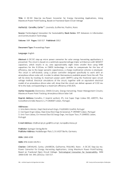
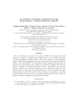
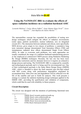
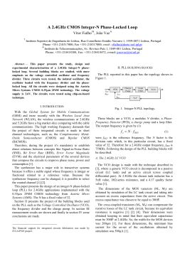
Revista Electrónica de Enseñanza de las Ciencias Vol. 9 Nº3, 569-595 (2010)
A study about the learning of students who worked
with computational modeling and simulation in the
study of simple electric circuits
Pedro Fernando Teixeira Dorneles, Eliane Angela Veit and Marco
Antonio Moreira
Federal University of Rio Grande do Sul – UFRGS, Physics Institute, Porto Alegre,
Brazil. E-mails: [email protected]; [email protected]; [email protected]
Abstract: The purpose of this research was to investigate the learning of
students who worked with computational modeling and simulation using the
software Modellus in the study of simple electric circuits. The theoretical
framework was based on Ausubel’s theory of meaningful learning and
Halloun’s schematic modeling approach. The quantitative results show that
there were statistically significant differences in the performance of students
who worked with the computational activities (experimental group), when
compared to the one in which students were just exposed to a traditional
method of teaching (control group). The qualitative results suggest that
many students from the experimental group seemed to have achieved
meaningful learning, and the students’ interaction among themselves and
with the teacher as well during the computational activities has strongly
contributed for that.
Keywords: computational simulation, computational modeling, learning
difficulties, simple electric circuits, physics teaching.
Introduction
It is common sense, nowadays, that engagement and interactivity are
decisive factors to learning. The studies of Beichner (1990), Redish and
Wilson (1993), Hodson (1994), and Beichner y Saul (2003), for example,
show that active participation in classes and interactivity with instructional
materials are key-points for the students’ learning. According to Beichner y
Saul (op. cit.), an active learning environment provides more favorable
conditions for students to acquire a better conceptual understanding and to
become more skillful in the resolution of physics problems.
In the teaching of simple circuits, which is the object of this research, the
most traditional way of fostering engagement and interactivity comprises
the development of experimental activities that take into account the
students’ previous knowledge (e.g., Shaffer y McDermott, 1992). More
recently interactive simulations as Physlets (2009) and PHET(2009),
providing a bridge between the static figure and the physical word (Cox,
Belloni y Christian, 2005), and integration between experimental and
computational activities (Ronen y Eliahu (2000); Zacharia y Anderson
(2003), Finkelstein, Adams, Keller et al. (2005)), besides motivating the
students, contributed to the meaningful learning of electric circuits. The
drawing of concept maps and V diagrams (Novak y Gowin, 1984; Moreira,
2006) are some of other instructional techniques applied to promote
569
Revista Electrónica de Enseñanza de las Ciencias Vol. 9 Nº3, 569-595 (2010)
interactivity. The present study also integrates experimental and
computacional simulation activities but in addition there are computational
modeling activities.
In the literature, acceptance attributed to activities of computational
simulation and modeling is not common sense. To our understanding, in
computational simulation activities, the student has autonomy to assign
initial values to the variables, to change parameters, but he/she does not
have autonomy to modify the core of the computational model, that is, the
access to its most basic elements, mathematical or iconical. In
computational modeling activities, in addition to being able to act upon the
parameters and initial values, the student has access to such basic
elements. Computational modeling activities are usually classified in two
ways: exploratory and expressive (or creative). In the exploratory activities,
the individual works with computational versions of scientific models and
representations (graphs, animations, tables, diagrams) developed by other
people and then they explore them through the most diverse perspectives.
In the expressive activities, the individual designs his/her own
computational models and creates ways to represent them.
Among the many computational tools available (Interactive Physics, Java
applets, Stella, PowerSim, Modellus, etc.), we selected the software
Modellus (Teodoro, Vieira y Clérgio, 2008), because with this software it is
possible to propose both types of activities (simulation and modeling) and
both ways of interaction of students with the computational model
(exploratory and expressive). Besides, Modellus has an intuitive interface
that facilitates the interaction of students with computational models in real
time allowing them the observation of multiple conceptual experiments
simultaneously.
Nowadays Modellus has started being very much used in teaching
activities (e.g., Teodoro, 2008, Advancing Physics, 2004), however, in
literature, studies that systematically look for the benefits of using such tool
in relation to students’ learning are scarce. Araujo, Veit y Moreira (2008)
carried out a study about the use of computational simulation and modeling
activities with Modellus presented in the form of problem-situations as an
instructional complement in the teaching of kinematics graphs. This
research involved two groups of students (experimental and control groups)
who had already been exposed to formal instruction in kinematics and it
was developed as an extra-class course. An adaptation to Portuguese of the
“Test of Understanding Graphs in Kinematics” TUG-K (Beichner, 1994) was
used to evaluate the conceptual understanding of the students; results
show that there were statistically significant improvements in the
performance of the students of the experimental group, when compared to
the control group exposed to a traditional method of instruction. This finding
suggested that the use of computational activities could improve the
students’ ability to understand kinematics graphs. An important aspect was
that the students presented more willingness to learn because during the
interactions with the computational models they realized the relevance of
some mathematical relations and physics concepts, and the concepts that
had previously seemed abstract became more familiar and concrete. These
results encouraged us to carry out the present research, which differs from
the former one by Araujo, Veit y Moreira (2008) in terms of the physics
570
Revista Electrónica de Enseñanza de las Ciencias Vol. 9 Nº3, 569-595 (2010)
content and for having been developed during class periods of a regular
discipline of the Engineering course, that typically is attended by 40
students per class.
Learning difficulties in simple electric circuits
Electricity is one of the areas of physics most studied in terms of learning
difficulties. A significant part of these studies refers to the teaching of
simple electric circuits and, according to these studies, students even after
formal instruction are not able to analyze and predict the behavior of
physics magnitudes involved in such circuits. In our literature review
(Dorneles, 2005) we included the main journals on physics teaching, from
1985 to 2005 in which we found 44 publications about learning difficulties of
simple electric circuits, and among those, we point out three: McDermott
and Shaffer (1992), Duit y Von Rhöneck (1998) and Englehardt y Beichner
(2004).
MacDermott y Shaffer (1992) carried out a systematic longitudinal study
to identify students’ difficulties in the learning of simple electric circuits. It
involved students who had never had physics classes before, students who
had completed a specialization course or had already teaching experience,
together with two large groups of college students enrolled in the
introductory courses of Calculus and Algebra. Results indicate that
conceptual difficulties and misconceptions presented by the students as
they analyzed an electric circuit seem to vary in difficulty and frequency. It
was detected that with formal instruction some difficulties tend to
disappear, while others may persist indefinitely and hinder students’
learning of more advanced topics. McDermott y Shaffer (op. cit.) classify
mistakes made by students during the study of simple electric circuits into
three categories: inability to apply formal concepts to electric circuits;
inability to use and interpret formal representations of an electric circuit;
and inability to qualitatively argue about the behavior of an electric circuit.
In a second study (Shaffer y McDermott, 1992), a tutorial was developed
based on laboratory instructional strategies to help students overcome their
difficulties. This tutorial was tested, modified and reviewed through
continuous evaluation based on experiments carried out in the classroom.
Its efficacy was compared to traditional teaching in a study involving 600
university students. Results seemed to show significant differences in the
conceptual understanding of the students who had used the tutorial
compared to the ones exposed only to traditional teaching. In both cases,
students able to solve the quantitative problems were often unable of
conceptually analyze the same electric circuit, whereas students of the
tutorial classes solved substantially better all the qualitative problems
proposed. The tutorial materials also seemed to be more effective for
overcoming some misconceptions. We point out the relevance of these
studies (Shaffer y McDermott) because besides contributing with the
identification of main learning difficulties, they also helped verify how
students progressed along the study of electric circuits, as well as
presenting a pedagogical proposal for helping overcome those hindrances.
Duit y Von Rhöneck (1998) presented a synthesis of research results that
show before and after instruction conceptions in the domain of electricity.
They emphasized the teaching of simple electric circuits and identified the
571
Revista Electrónica de Enseñanza de las Ciencias Vol. 9 Nº3, 569-595 (2010)
role of students’ pre-instructional conceptions in the teaching/learning
process, while distinguishing between misconceptions and the conceptions
that serve as a basis for the students’ development of an adequate
understanding. The students’ learning difficulties in the field of electricity
serve as example for Duit y Von Rhönech (op. cit.) to point out the
importance of students’ pre-instructional conceptions in the learning of
physics.
Engelhardt y Beichner (2004) developed a multiple choice test with 29
questions to detect and interpret concepts about direct current resistive
electric circuits (DIRECT – Determining and Interpreting Resistive Electric
Circuit Concepts Test), that has been used with hundreds of students of
secondary and university levels in the United States and Canada. There are
two versions, the first (version 1.0) was applied to 1135 students and the
second (version 1.1), to 695. The results show that both versions may be
useful in the evaluation of curriculum or instructional materials. Version 1.0
is more qualitative, seeming more adequate to identify misconceptions,
while version 1.1 is more quantitative, seemingly more adequate to identify
students’ mathematical skills. Many of the difficulties identified by
Engelhardt y Beichner (op. cit.) with the application of the two versions of
the DIRECT test are similar to the ones identified in the studies of
McDermott y Shaffer (1992) and of Duit y Von Rhöneck (1998).
Learning difficulties presented in these three studies may be classified as
conceptual difficulties, misconceptions and indiscriminate use of mistaken
language and reasoning. Table 1 presents a synthesis of the difficulties of
specific nature related to the concepts of electric current, potential
difference and electric resistance, and the main misconceptions derived
from these references.
The indiscriminate use of language is considered a hindrance to learning
because the meanings associated to physics concepts by the students are
frequently different from those that a physicist attributes to the same
concept. For example, the meanings attributed to the concept of electric
current in everyday language include a broad range of meanings about
energy quite different from those scientifically accepted for this physics
concept. The mistakes in a physics class, consequently, are common, and
even more frequent if the teacher is not aware of the difference between
his/her own context and the one of the students when talking about electric
phenomena (Duit y Rhöeneck, 1998, Pacca, Fukui y Bueno et al, 2003).
The students who presented faulty reasoning in the study of simple
electric circuits seem to tend to develop sequential or local reasoning
instead of a systemic one. According to McDermott y Shaffer (1992),
students who present sequential reasoning analyze a circuit in terms of
“before” and “after” the flow of an electric current, that is, they recognize
that a change in the “beginning” of the circuit influences the subsequent
elements, although they consider that a change at the “end” of the circuit
does not influence “former” elements.
572
Revista Electrónica de Enseñanza de las Ciencias Vol. 9 Nº3, 569-595 (2010)
Conceptual difficulties
Misconceptions: The students…
Electric current
1. To consider the conservation of a) … think that the current is consumed
the electric current.
passing through an electric resistance (12. To understand that intensity of an 3).
electric current in a circuit depends on b) … think that the battery is a source of
characteristics of the source, but also constant electric current (1-3).
on the equivalent resistance of what c) … believe that the order of the
has been coupled between their elements in the circuit and the direction of
terminals.
the electric current are relevant (1-3).
3. To recognize that the intensity of d) … think that the source provides the
the electric current does not depend charge carriers responsible for the electric
on the order in which the elements in current in the circuit (3).
the electric circuits are found, or on
the direction of the current.
Electric resistance
1. To
distinguish
equivalent e) … often think of the equivalent
resistance of part of a circuit and the resistance
of the circuit as if were a
electric resistance of an individual property of an individual element of the
element.
circuit (1).
2. To realize that the equivalent f) … when determining how the electric
resistance is a useful abstraction for current divides itself into parallel branches
obtaining the total current or the of a circuit, consider only the number of
potential difference in part of a circuit. branches and not the relative electric
3. To understand that the electric resistances of the various branches (1-3).
current divisions at a junction point of g) … think that if a resistor reduces the
the circuit depend on the circuit current by x, two resistors will reduce it by
configuration.
2x,
independently
of
the
resistors’
4. To
understand
the
serial configuration (3).
association of resistors as a hindrance h) … consider that resistors aligned
to current flow; and the association in geometrically in series are associated in
parallel as an alternative for the series either if there is a junction or not
current flow.
between them; and that resistors aligned
5. To identify associations in series geometrically in parallel are associated in
and in parallel.
parallel even if there is a battery in the
branch (3).
Potential
1. To differentiate the concepts of
potential difference and of electric
current.
2. To differentiate the concepts of
potential difference and of electric
potential.
3. To recognize that an ideal battery
maintains
a
constant
potential
difference between its terminals.
4. To
calculate
the
potential
difference between pairs of points
along the circuit.
difference
i) … think about the battery as a
constant source of electric current and not
as a source of constant potential difference
(1-3).
j) … understand the potential difference
as a property of the electric current (3).
k) … consider that the potential difference
between pairs of points along the circuit
remains constant (1).
l) … associate brightness of a light bulb
to the potential value of one of the
terminals of the bulb (2).
Table 1.- Synthesis of the conceptual difficulties and alternative conceptions
identified in the third column by (1) Duit y Von Rhöneck (1998), (2) McDermott y
Shaffer (1992) and (3) Engelhardt y Beichner (2004).
573
Revista Electrónica de Enseñanza de las Ciencias Vol. 9 Nº3, 569-595 (2010)
The students who present local reasoning focus their attention on a point
of the circuit as they ignore the rest of the electric circuit. For example,
when analyzing the electric current divisions at a point of the junction
(current divisor) of a circuit containing many parallel branches, students
seem to despise what exists in each branch and consider that the electric
current divides itself into equal parts in each branch of the circuit (Duit y
Rhöenck, 1998).
Another difficulty often reported in the literature, especially in studies
that involve secondary students, is the inability to apply the concept of
complete circuit. For example, many students are not able to turn on a light
bulb with a battery and one single electric wire, since they do not consider
that a light bulb has two terminals (bornes) for establishing a connection
(Arnold, Middle y Millar, 1987; Sanchez y Sánchez, 1989; McDermott y
Shaffer, 1992; Shepardson y Moje, 1994; Benseghir y Closset, 1996;
Chambers y André, 1997; Shepardson y Moje, 1999; Sencar y Eryilmaz,
2004; Chiu y Lin, 2005).
Table 2 presents the other studies found in our literature review
(Dorneles, 2005) and the main conceptual difficulties, misconceptions and
mistaken reasoning found or mentioned in each study.
Theoretical framework
The theoretical framework of this research is anchored in Ausubel’s
(1978; 2000) theory of meaningful learning and in Halloun’s schematic
modeling approach (Halloun, 1996). From Ausubel we took into account the
role of previous knowledge, progressive differentiation, integrative
reconciliation, and conditions for the occurrence of meaningful learning.
Ausubel’s theory is a constructivist cognitive theory directed to learning the
way it happens in the classroom, everyday in most schools. To Ausubel
(1978, p.iv), “The most important single factor influencing learning is what
the learner already knows. Ascertain this and teach him accordingly”. New
concepts may be learned and retained as relevant and inclusive concepts
are adequately clear and available in the cognitive structure of the
individual serving as anchorage to new ideas and concepts. Progressive
differentiation and integrative reconciliation are two programmatic principles
that refer to classroom dynamics. Progressive differentiation is the principle
according to which the most generic and inclusive ideas of the teaching
topic should be presented at the beginning of teaching and then they can be
progressively differentiated in their details and specificities (Moreira, 2006).
To Ausubel (2000), there are two conditions for meaningful learning to
happen: i) the material must be potentially meaningful, that is, the content
to be studied must be relatable to the students’ cognitive structure in a
non-arbitrary and non-verbatim way; ii) the students must have willingness
to relate the new potentially meaningful material in a substantive and nonarbitrary way to their cognitive structure.
574
Revista Electrónica de Enseñanza de las Ciencias Vol. 9 Nº3, 569-595 (2010)
Reasoning
Conceptual Alternative
difficulty
conception Local Sequential
Andrés (1990)
2.1
Axt y Alves (1994)
1.1
Barbosa, Paulo y Rinaldi (1999)
1.1
a)
X
1.1
a)
Carter, Westbrook y Thompkins
(1999)
Castro (1992)
2.1
Dupin y Johsua (1987;1990)
2.3
b)
Dupin y Johsua (1989)
1.2
Gravina y Buchweitz (1996)
1.1
a)
2.1
Gutwill, Frederiksen y Ranney
(1996)
2.1
Liegeois, Chasseigne, Papin et
al.(2003)
Liegeois y Mullet (2002)
2.1
X
Metioui, Brassard, Levasseur et al
(1996)
Miera, Rosado y Oliva (1991)
1.1
a)
Millar, Beh y Alam (1993)
2.1
Millar y King (1993)
2.1
Moreira y Domínguez (1987)
1.1 e 1.2
a) e f)
Nieto, Campo y Martinez (1988)
1.1 e 2.1
a)
x
Olde y Jong (1990)
1.1
a)
1.1
Paatz, Ryder, Schwedes et al
(2004)
Pardhan y Bano (2001)
1.1
Psillos (1988)
2.1
Saxena (1992)
3.3
j)
x
1.1 e 2.1
a)
x
x
Shipstone, Rhoeneck, Jung et al.
(1988)
Silveira, Moreira y Axt (1989)
1.1
a)
Solano, Gil, Pérez et al. (2002)
1.1
f)
x
Stocklmayer y Treagust (1996)
1.1 e 2.1
Talim y Oliveira (2001)
1.1
Tsai (2003)
1.1
a)
1.1
a)
Vieira, Quillfeldt, Selistre et al.
(1986)
Webb (1992)
1.1
Studies
Table 2.- Research papers about the teaching of simple electric circuits. The
identification for the conceptual difficulties use the convention presented in table 1.
From Halloun (1996), we considered his proposal of schematic modeling
that may be applied to the solution of paradigmatic problems, defined as
those that possess special characteristics and whose solution cannot be
obtained through direct formula application and substitution of numerical
values, including open-ended questions. The solution of such problems
requires students to think about their own conceptions about the physics
system, thus favoring meaningful learning. Halloun’s schematic modeling
processes in five non-hierarchical stages: selection, construction, validation,
575
Revista Electrónica de Enseñanza de las Ciencias Vol. 9 Nº3, 569-595 (2010)
analysis and expansion. In the solution of a paradigmatic problem, the first
stage of the process consists of the selection of a scientific model from a
repertoire of familiar models of a specific theory. The selection is guided by
the domain of the model, the objective of modeling (i.e., of the problem)
and the validity of expected results (including approximations and precision
of results). Then, the solution of the problem is formulated by constructing
a mathematical model that takes into account relevant parameters, initial
conditions, constraint conditions; finally, a model that can be continuously
processed, analyzed and validated to evaluate if it leads to an acceptable
solution to the problem at study. These intermediate stages of construction,
validation and analysis juxtapose, and some of these steps occur
concomitantly. The expansion of the model includes a description or
prediction of new situations referring to the same system focused on, or
implications to other reference systems, as well as extrapolations for the
design of new models.
Methodology
Object of study and research hypothesis
This study investigated the learning of students who worked with
computational simulation and modeling presented as a problem situation
proposed though the software Modellus, in the teaching of simple electric
circuits. A problem situation consists of a particular situation in physics
upon which questions are made with the purpose of stimulating students to
think and interact consciously with computational resources and not merely
by trial and error.
As a research hypothesis we assumed that the use of computational
modeling and simulation activities as complements to the classroom and
physics laboratory activities can favor the students’ predisposition for
learning, by relating the new information in a substantive and non-arbitrary
way to his/her cognitive structure, thus, creating conditions for meaningful
learning of physics concepts involved in simple circuits. This could generate
better performance from the students in the posttest on the studied topic as
well as promoting better conditions for the students to attain specific
objectives (Table 3).
Design
This study was carried out when simple electric circuits concepts were
taught in the course of Physics II-C (Electromagnetism for Engineering
students of the Federal University of Rio Grande do Sul - UFRGS, Brazil).
193 Engineering students who attended the course in the second semester
of 2004 participated in the study. The experimental and control group were
randomly chosen. A class with 28 students formed the experimental group,
and 165 students, from five sections of the course in which the research
was carried out, formed the control group. The students of the experimental
group worked with computational simulation and modeling during the
teaching of simple electric circuits, whereas the control group was exposed
only to traditional teaching. Qualitative and quantitative evaluations were
applied to the students’ learning outcomes. As qualitative evaluation we
considered the students’ opinions about the treatment and answers to the
576
Revista Electrónica de Enseñanza de las Ciencias Vol. 9 Nº3, 569-595 (2010)
discursive questions presented in printed guides during the classes.
Quantitative evaluation was developed according to quasi-experimental
design (Campbell y Stanley, 1963) in which there is a non-equivalent
control group and an experimental group.
Procedures
Based on the learning difficulties presented in table 1 and in mistaken
reasoning students usually present, we established general and specific
objectives to be attained by students after the teaching of simple electric
circuits (table 3).
Given a
The student should…
... grasp:
1. that it is necessary to deal with the electric circuit as a
system;
2. the conservation of electric current in the electric circuit;
simple
General
3. the relation between total electric current and the
electric
resistances associated in the circuit;
objectives
circuit
4. the behavior of equivalent resistance to different
associations;
5. electric current as a consequence of potential difference
and electric resistance;
... grasp that:
a) the electric current that runs through the resistors is the
same;
resistors’
b) the sum of the potential difference between the
association
terminals of resistors is the same as the potential
in series
difference applied by the source;
c) equivalent resistance increases (diminishes) when a
resistor is inserted (taken out) in a series association;
... grasp that:
d) the potential difference between the ends of resistors is
the same;
resistors’
e) current divisions at a junction of the circuit (current
association
Specific
divisor) depend on what already exists in the rest of the
objectives in parallel
circuit;
f) the equivalent resistance decreases (increases) when a
resistor is inserted (taken out) in a parallel association;
… be able to:
g) identify that a light bulb is a resistor and, therefore, the
light
bulb
observed behavior in relation to resistors is also
circuits
manifested in light bulbs;
h) associate the brightness of a light bulb to electric
current;
ideal
i) … grasp that an ideal battery is not a source of constant
electric current, but a source of constant potential
tension
difference.
source
Table 3.- General and specific objectives to be attained by the students when
working with computational simulation and modeling about simple electric circuits.
To help students achieve the objectives presented in table 3, we designed
a series of simulation and modeling computational activities (Dorneles, Ives
y Veit, 2005) as an instructional resource. For each activity we developed
577
Revista Electrónica de Enseñanza de las Ciencias Vol. 9 Nº3, 569-595 (2010)
material containing: objectives to be attained by the students, a general
description of the model, and a printed guide with discursive questions to be
answered by the students in class.
The treatment adopted in this study comprised the implementation of
designed computational activities, using the collaborative methods, in which
the teacher presents the most general ideas of the subject matter in an
introductory explanation, typically of 30 to 40 minutes, out of a 1h40min
total period, to be progressively differentiated in terms of details and
specificities. After the introductory lecture, the students, in small groups of
2 to 3 partners engage in computational activities. For each group there is
one PC and the accomplished tasks are handed in by the end of each class
for formative evaluation purposes. With the requirement of handing in just
one copy per group, we expect to promote the negotiation of meanings
among the students, who are committed to finding a solution that complies
with the ideas of all members of the group. The small and large group
discussions favor students’ interaction among themselves and with the
teacher, who acts as mediator in the interaction between computer and
learner and in the internalization of meanings by the learner (Vygotsky,
2003). Reflection, interaction, and engagement are encouraged with the use
of a method we can call PIE – Predict, Interact, Explain – adapted from the
POE method – Predict, Observe, Explain – proposed by White and Gunstone
(apud Tao y Gustone, 1999), which consists of describing problemsituations in physics, or of presenting them through visual demonstrations,
video projections or, as discussed here, computational simulations so as to
help students predict what might happen. Then, opportunity is given to
them to interact with the computational resource in order to generate
results and evaluate what can effectively happen and, finally, to explain the
differences and similarities between their ideas and the scientific solutions
already accepted for the problem-situation at issue.
Treatment
The treatment was applied to a total of five classes of 1h40min each in
the computer laboratory, where the students from the experimental group
worked in pairs with computational simulation and modeling. At the
beginning of each class the students received printed guides with discursive
questions to be answered in groups with the PIE method. At the end of the
class, each group handed in a single copy of the guide containing
consensual group answers for evaluation purposes. From the second class
on, we began each class with a coordinated discussion (~ 15 minutes) with
all the students about the activities performed in the previous class.
Evaluation tools for students’ learning
In the present study we have chosen to apply the test on simple electric
circuits as proposed by Silveira, Moreira y Axt (1989), transcribed in
Apendix A, because it is well accepted among teachers who have already
taught the subject matter that is the focus of this study. Then, it had
provided us a large control group. Furthermore, the reliability coefficient of
the instrument (Cronbach’s alfa) was calculated for a target population
seemingly similar to ours (Silveira, Moreira y Axt, op. cit.). Since the
578
Revista Electrónica de Enseñanza de las Ciencias Vol. 9 Nº3, 569-595 (2010)
reliability coefficient is not a property exclusively associated to the
instrument, but a property of it pertaining to a certain group, we
recalculated the reliability coefficient of the test, that will be presented in
the next section.
We applied this instrument as a pre-test both in the control and the
experimental groups in the first day of classes to verify learning difficulties
measured by this test as well as to use them as a covariable for the analysis
of the results of the post-test. That test was applied to both groups at the
end of classes about electric circuits to verify possible effects of the
treatment. It took students approximately 30 minutes to answer the tests,
and the application interval between the pre-test and the post-test was of
seven weeks.
Results and discussion
Reliability analysis of pre and post-tests
We calculated the reliability coefficient of the test proposed by Silveira,
Moreira y Axt (op. cit.) before (pre-test) and after (post-test) the teaching
of simple electric circuits based on the answers of students who attended
the course Physics II-C, in the semester in which we carried out the present
study, but who did not participate in the experimental or control group. The
internal consistence analysis (ICA) was carried out according to Cronbach
(1967, apud Moreira y Silveira, 1993). The ICA included the calculus of the
Cronbach’s alpha coefficient, whose result is presented in table 4, together
with the correlation coefficient of the score of each item with the total score.
In both cases the coefficients were higher than 0.7, showing the capacity of
the test to discriminate students with scientific conceptions from those with
misconceptions about simple electric circuits.
N
Total score
average
Standard deviation
of the total score
Items
Cronbach alfa
coefficient
Pre-test
66
7.70
2.82
13
0.75
Pos-test
53
8.36
3.25
13
0.85
Test
Table 4.- ICA synthesis for the test on simple electric circuits applied to
engineering students before and after instruction.
Comparison between the experimental and control group
The percentages of correctness of each item of the pre-test and of the
post-test of the experimental and control group are presented in table 5.
The data referring to item 8 of the test were not part of our analysis, for it
involves a RC circuit, and when we applied the post-test the students had
only studied the simple circuits. We can observe that for both groups the
percentage of correctness of each item in the post-test is higher than the
one presented in the pre-test.
579
Revista Electrónica de Enseñanza de las Ciencias Vol. 9 Nº3, 569-595 (2010)
Objectives* Item
a)
Experimental group (28
students)
Correct items
(Pre-test)
Control group (165
students)
Correct items Correct items Correct items
(Pos-test)
(Pre-test)
(Pos-test)
82
100
89
90
a)
1
2
14
86
53
59
e)
3
39
64
56
67
c), e)
4
18
43
38
41
-
5
18
79
55
64
e)
6
29
86
47
54
a)
7
21
25
29
28
9
10
11
12
13
14
71
71
11
0
61
36
100
79
57
57
75
68
88
89
15
16
79
39
90
90
18
21
84
42
a)
e)
f)
f)
a), e)
a), c), e)
Table 5.- Students’ performance from the experimental and control group on the
pre and post-tests. In the first column, we indicate the specific objectives measured
for each item of the test. *The objectives g) and h) pervade all the test’s items.
In table 6 we observe the total score averages of the experimental and
control groups in the pre-test and in the post-test. In the pre-test, the
control group average (6.94) was higher than the average of the
experimental group (4.71); the statistical level of significance of the
difference between the averages was less than 0.01. We also did a Variance
and Covariance Analysis – ANOVA/ANCOVA (Finn, 1997). Table 7 shows the
adjusted average in the post-test to both groups, and also the ratio F of
Snedecor (through which the level of statistical significance is obtained) for
the difference between the two averages and the level of statistical
significance of this difference.
Pre-test
Total
Group
score
average
Experimental
4.7
Control
6.9
Pos-test
Standard
deviation
Correct
answers
2.5
2.7
36%
53%
Total
score
average
9.2
7.5
Standard
deviation
Correct
answers
2.4
2.7
71%
58%
Table 6.- Comparison between experimental and control groups in the averages
of the pre-test and post-test. Maximum score = 13.
Group
Experimental
Control
Adjusted average
in the post-test
10.2
7.3
F
Level of statistical
significance
38.7
0.000
Table 7.- Comparison between the experimental group and control group of the
adjusted averages of the post-test.
Based on the comparison between the average performance of the
experimental and the control group in the adjusted averages of the post-
580
Revista Electrónica de Enseñanza de las Ciencias Vol. 9 Nº3, 569-595 (2010)
test (Table 7), we used the null hypothesis, concluding that the average
performance of the students who worked with computational simulation and
modeling was higher than that of the other students, with a level of
statistical significance lower than 0.01.
To compare the performance of the two groups in terms of the objectives
measured through the test, we compared the gain of the experimental and
control groups in the average scores of the questions associated to each
specific objective (column 1 table 5), the level of statistical significance
being obtained with the U-Test of Mann-Whitney (a non-parametric test
equivalent of the t-test to the average difference). The results are shown in
table 8, in which we can observe that for every objective analyzed the
performance of the students from the experimental group was higher than
the one of the control group, with a level of statistical significance lower
than 0.01.
Group
Experimental Average
Average standard error
Control
Average
Average standard error
Level of statistical significance
Gain a) Gain c) Gain e)
1.68
0.57
1.61
0.27
0.18
0.32
0.15
0.05
0.29
0.10
0.06
0.10
0.000
0.002
0.000
Gain f)
1.04
0.18
0.08
0.07
0.000
Table 8.- Comparison between the experimental and the control groups in terms
of each specific objective (column 1 table 5). The level of statistical significance was
obtained through the U-test of Mann-Whitney.
To illustrate the simulations developed with the students, in table 9 and
in figures 1 to 3 we present in detail the computational activity that helped
students attain objectives a), c) and e). In this activity, the students initially
answered questions 1 and 2 from table 9 to make predictions about the
behavior of the equivalent resistance and of the electric current shown in
figure 1. Then, they interacted with animation 2 (Figure 2) to generate
results, and afterwards they evaluated the divergences and convergences of
their predictions (question 3 from table 9). Finally, they answered four
conceptual questions about the potential difference along the circuit shown
in figure 3 (questions 4 to 7 from table 9).
Qualitative analysis of the answers of the students of the experimental
group to questions 1 to 3 of table 9 agrees with the quantitative results
related to objectives a), c) and e) (Table 3). Following, we present some
examples of the students’ answers.
Answers to question 1, related to objectives c) and e):
The equivalent resistance decreases because the current does not pass
through R1 anymore, for the segment of the wire that passes through
A has negligible electric resistance, which turns it preferable. We
noticed that because of the increase of the total electric current when
we closed switch A-B (Group 2).
As we close switch A-B, the electric current does not pass through R1
anymore and the resistance in the whole circuit decreases. The electric
current tends to follow what makes less electric resistance easier
(Group 6).
581
Revista Electrónica de Enseñanza de las Ciencias Vol. 9 Nº3, 569-595 (2010)
The equivalent resistance of the circuit goes down with the switch in
position A, the electric current passes all through the new path,
increasing the amperage (current) in the circuit (Group 15).
General description
Running the model and changing the position of the switch shown in figure 1, an
ammeter registers an electric current variation at a specific point of the circuit,
through which the total current of the circuit (It) runs. With the help of the
ammeter (Figure 2), it is possible to observe the behavior of the electric current
along the circuit and with the voltmeter (Figure 3), it is possible to observe the
potential difference between many pairs along the circuit.
Objectives of the activity
1) given a potential difference between two points of a simple circuit, the
student should: a) be able to understand the electric current as a consequence
of the potential difference and the electric resistance; b) relate the increase of
electric current in the circuit to the decrease of the equivalent resistance;
2) given a junction of the circuit (current divisor), the student should notice
that the division of currents depends on what is connected in the circuit;
3) given an association of resistors in series, the student should realize that:
a) the current that runs between them is the same; b) the equivalent resistance
increases when a resistor is associated in series; c) the sum of the potential
difference between the ends of resistors is the same as the potential difference
applied between the ends of the source; d) the potential difference applied
between the ends of the source is an intrinsic characteristic of the source; e) it
is necessary to deal with the circuit as a system.
Questions proposed to the students
1) Run the model and answer the following question: closing the switch A-B,
what happens to the equivalent resistance shown in Animation 3? Why?
2) The intensity of the electric current in point E, in relation to the intensity
measured in the ammeter is: a) lower; b) equal; c) higher
3) Open Animation 2. Verify prior answers. What can be said about the
behavior of the electric current in the circuit?
4) Open Animation 1. On the right side of the animation window there are
voltmeters to measure the potential difference between different pairs of points
of the circuit. Modify the value of the electric resistance of the resistors. When
switch A-B is in position B and the resistors R2 and R3 in the maximum value,
what is the potential difference between points b-d?
5) When switch A-B is in position A and the resistors R2 and R3 are at their
lowest values, what is the potential difference between points a-d?
6) When switch A-B is in position B, click with the left button of the mouse
over the analogic meter of R4 and inform the value 1000 (value in ohms). To
which values tend the electric current and the potential difference between
points d-e? Why?
7) Is it possible to modify the potential difference (V) between the ends of the
source at any position of switch A-B? Why?
Table 9.- Detail of a computational activity that helped students attain specific
objectives a), c) and e) presented in table 3.
582
Revista Electrónica de Enseñanza de las Ciencias Vol. 9 Nº3, 569-595 (2010)
Figure 1. – Screenshot: Animation 3 of the computational simulation presented
in table 9.
Answers to question 2, related to objective a):
In an association in series, the intensity of the electric current is the
same at all points (Group 11).
The electric current does not vary, it remains the same along the
circuit (Group 13).
The electric current remains the same in an association in series
(Group 15).
Figure 2.– Screenshot: Animation 2 of the computational simulation presented in
table 9.
583
Revista Electrónica de Enseñanza de las Ciencias Vol. 9 Nº3, 569-595 (2010)
Figure 3.– Screenshot: Animation 1 of the computational simulation presented in
table 9.
These results suggest strong indications that the computational
simulation presented in table 9 has helped students overcome a
misconception according to which the electric current is consumed when
passing through an electric resistance. Other important result is that by
varying a parameter in a circuit students could instantaneously observe
alterations along the circuit, which motivated them to develop systemic
reasoning, that is, to deal with an electric circuit as a system. For example,
many students while analyzing the current division at a point of junction of
the circuit did not apply local reasoning, that is, they did not focus their
attention on just one point of the circuit; quite the contrary, they
considered the divisions of electric current at a point of junction of the
circuit to depend on what already existed in the whole of the circuit.
Since none of the test items adequately measures objective b), we
qualitatively analyzed question 6 from table 9. The results suggest that a
few students have reached such objective, since only three groups, from a
total of 15, have presented clear argumentation based on the concept of
potential difference, which will be transcribed next.
The electric current tends to zero because resistance R4 is too high,
the higher the resistance, the lower the electric current. The potential
difference between d-e tends to the maximum value 20V (Group 10).
It is that the total electric current tends to zero (0.002A) and V tends
to the maximum (20.0V), because resistance increases, decreasing the
electric current” (Group 9).
The electric current tends to zero because the higher the resistance
the lower the electric current. And the potential difference tends to
20V, which is the maximum value, because, as resistance is increased,
the potential difference between the two points also increases (Group
11).
584
Revista Electrónica de Enseñanza de las Ciencias Vol. 9 Nº3, 569-595 (2010)
This result may not necessarily mean that computational simulation did
not contribute to a better understanding of the students about potential
differences in an association of resistors in series, but that the question
proposed might not be appropriate for this evaluation. The instructional
material could be more efficient in relation to this objective if it included
questions that would necessarily require students to apply the concept of
potential difference.
As for the objective d), we have qualitatively analyzed the students’
answers to question 1) of the computational simulation described in table
10 whose main screen is presented in figure 4. We have found strong
indications that the majority of students reached such objective. In their
own words:
The currents I1 and I2 remain constant since the resistors are in
parallel and the total current changes. When the value of R3 is greater,
It it decreases and when R3 is lower, It it increases (Group 10).
I1 and I2 remain constant because R1 and R2 and the tension are
constant, and the current depends on these parameters. It diminishes
with the increase of R3, for this increases the total resistance of the
circuit (Group 2).
Circuit in parallel (V=cte) altering the value of R3 (decreasing) more
current passes through it, I is proportional to 1/R (Group 3).
Figure 4.– Screenshot: Animation 1 of the computational simulation described in
table 10.
585
Revista Electrónica de Enseñanza de las Ciencias Vol. 9 Nº3, 569-595 (2010)
General description
By running the model, it becomes possible to obtain two or three resistors
associated in parallel, by varying the position of the switches. There is still the
possibility of associating them in series with a fourth resistor. The ammeter
registers the electric current that passes through each resistor at any position of
the switches. We can modify the value of the electric resistance in the resistors
and the potential difference between the ends of the source, as shown in figure 4.
Objectives of the activity
Given a circuit with resistors of mixed association, the student should be able to:
a) deal with the circuit as a system; b) notice the behavior of the equivalent
resistance; c) identify the behavior of potential difference on the ends of the
resistors; d) identify what is the intensity of electric current that passes through
each resistor.
Questions proposed to the students
1) With the switches at positions A and D, modify the value of R3. Explain the
behavior of the values of i1, i2 and it.
2) With the switches at positions A and C, modify again R3. Explain why, in this
case, all the currents vary.
Table 10.- Details of a computational activity which helped the students attain
the specific objectives d) and I) presented in table 3.
Another important aspect is that interacting with the computational
simulation described in table 10, many groups (13) did not apply sequential
reasoning and did not analyze the electric circuit in terms of “before” and
“after” the passage of electric current; quite the contrary, they dealt with
the circuit as a system and were able to recognize that an alteration in one
parameter of the circuit causes instant alterations along the circuit.
Following we present how the students from group 14 answered question
b).
Once R1, R2 and R3 are associated in parallel, the potential difference
must be the same in each one. Diminishing R3, I3 increases and
consequently I4 becomes higher. For that, potential difference in R4
will have to be higher, because R4 remains equal. That’s why the
potential difference of the resistances in parallel will change (will be
lower) what makes I1 and I2 also change (Group 14).
As for objective i), just three groups, when working with the
computational activities proposed in this study, presented the
misconception that an ideal battery is a source of constant electric current;
the others, 12 groups, seemed to have reached the objective, that is,
considered that the intensity of an electric current of a circuit does not
depend only on the characteristics of the source but also on the equivalent
resistance of what has been coupled between its ends, and that an ideal
battery is a source of constant potential difference. Following, we show two
examples of each case:
First case:
The total electric current in an association in parallel is equal to the
sum of the currents in all the resistors. If you take out one resistor
from the association, the remaining ones will have a greater current
(Group 11 ).
586
Revista Electrónica de Enseñanza de las Ciencias Vol. 9 Nº3, 569-595 (2010)
In a circuit associated in parallel, the partial currents added result in
the total current. Since we have eliminated one resistor, the current
that passed through it will be added to the other resistors” (Group 2).
Second case:
Since the resistors R1, R2 and R3 are associated in parallel, the
currents I1 and I2 do not depend on the electric resistance of R3,
that’s why they remain constant as R3 is modified. The total electric
current increases with the decrease of R3, because by decreasing R3,
Req diminishes, while increasing the intensity of the total electric
current. The potential difference between the resistors is constant for it
depends only on source characteristics (Group 11).
In this case (the three resistors are associated in parallel) the currents
I1 and I2 remain constant when the electric resistance of R3 is altered
and the potential difference remains the same in all resistors(Group
13).
In synthesis, we have strong indications that the computational activities
developed in this research helped the experimental group students attain
the objectives related to the concepts of electric current and electric
resistance. However, it did not show efficiency in helping them to reach the
proposed objectives for potential difference. Many students, even after the
treatment, showed difficulties in understanding the decrease on potential
difference across an association in series.
In the next topic, we present some of the students’ opinions about the
treatment used in this study.
Raising opinions
We have also tried to evaluate our research hypothesis by analyzing the
students’ opinions about the treatment. The raising of students’ opinions
was encouraged by electronic mail during the second semester of 2005,
when the students had already received the final grade for the course.
Based on the analysis of the students’ statements we believe that the use of
computational activities may offer students opportunities for a better
conceptual understanding. On their own words they stated:
The use of computers facilitated understanding of the studied physics
phenomena. Simple use of the blackboard to explain the subject rarely
brings about clarity to physics concepts and with the simulations we were
able to observe everything that could possibly happen (Student 5).
It was easier to learn by visualizing what happened each time we
changed something in the circuit (Student 1).
I remember that after the simulations on the screen, the laws became
clearer, it was cool to see the resistors influencing
the circuit!
(Student 2).
It was quite nice to study in the computers, it made the content
clearer (Student 9).
Moreover, we believe that treatment is a motivational factor for
improving the students’ learning. On their own words:
587
Revista Electrónica de Enseñanza de las Ciencias Vol. 9 Nº3, 569-595 (2010)
The simulations give us a concrete view of what we learn theoretically
in class. The visualization of the circuits makes learning much easier,
stimulating and interesting (Student 3).
The development of assignments during the classes contributed a lot
to learning because by interacting with the simulations we had a very
good view of the physics concepts and moreover, with pair work, we
had the chance of discussing the observations right there and clearing
out doubts (Student 5).
I point out the disposition in the assistance of the student, always
searching for ways to present the best way of learning, besides the
change from the classical and formal environment of a conventional
classroom to a room with computers and audiovisual resources
(Student 7).
The computational activities proposed brought about many doubts,
sometimes the simulation itself answered the doubt, or we would ask
the teacher (Student 4).
These results seem to show that the computational activities developed in
this study can offer better conditions for meaningful learning of electric
circuits.
Conclusions
Nowadays, studies that identify learners’ difficulties with some contents
of physics have not been restricted just to the detection of difficulties, but
they also present alternatives to help students overcome them. We worked
with simple electric circuits, because many research results (e.g. McDermott
y Shaffer, 1992; Duit y Rhöeneck, 1998 and Engelhardt y Beichner, 2004)
show that many students even after being taught this topic, continue with
some misconceptions and mistaken reasoning. In order to help students
overcome such difficulties, McDermott et al. proposed some experimental
activities. In this study, we present as an alternative to overcome these
difficulties the use of computers. So, we developed computational
simulation and modeling activities that were designed taking into account
difficulties commonly experienced by students in the learning of electric
circuits to be worked in class with the PIE (predict, Interact, Explain) and
the use of collaborative methods.
The quantitative results of this study showed that there was a statistically
significant difference in the performance of students from the experimental
group, in comparison with that of the control groups, leading us to believe
that computational simulation and modeling activities can help students
overcome their learning difficulties usually faced when they study simple
electric circuits. The results of our qualitative analysis show that the
conceptual questions presented in the guides which require constant
students’ interactions with the computational models, might have promoted
the students’ predisposition to learn by relating in a substantive manner to
their cognitive structure the physics concepts involved, thus, allowing for a
better conceptual understanding. The willingness to learn is one of the
conditions for meaningful learning. The other is that the material must be
potentially meaningful. We believe to have attained both of these conditions
588
Revista Electrónica de Enseñanza de las Ciencias Vol. 9 Nº3, 569-595 (2010)
in this study, which agrees with Araujo, Veit y Moreira (2008), Ronen y
Eliahu (2000) and Finkelstein, Adams, Keller et al. (2005) whose findings,
suggested that the use of computational activities can improve conceptual
understanding while being itself a motivational element for learning.
We conclude pointing out that by using computational activities in the
teaching of electric circuits we are not proposing them as a replacement for
laboratory classes, but we believe we are increasing the range of
possibilities for helping students overcome their learning difficulties.
Thanks
We thank Prof. Dr. Fernando Lang Silveira for his contribution in the
statistic analysis of the results. This study is partially financed by CNPq,
National Brazilian Council of Technological and Scientific Development.
References
Andrés, M.M. (1990). Evaluación de un plan instruccional dirigido hacia la
evaluación de las concepciones de los estudiantes acerca de circuitos
eléctricos. Enseñanza de las Ciencias, 8, 3, 231-237.
Araujo, I.S., Veit, E.A. y M.A. Moreira (2008). Physics students’
performance using computational modelling activities to improve Kinematics
graphs interpretation. Computers & Education, 50, 4, 1128-1140.
Arnold, M., Middle, W. y R. Millar (1987). Being constructive: An
alternative approach to the teaching of introductory ideas in electricity.
International Journal of Science Education, 9, 5, 553-563.
Ausubel, D.P.
(2000). Acquisition and Retention of Knowledge: A
cognitive view. Dorchet: Kluwer Academic Publishers.
Ausubel, D.P., Novak, J.D. y H. Hanesian (1978). Educational psychology.
Nova York: Holt, Rinehart and Winston.
Axt, R. y Alves, V.M. (1994). O papel do voltímetro na aquisição do
conceito de diferença de potencial. Caderno Catarinense de Ensino de Física,
11, 1, 19-26.
Barbosa, J.O., Paulo, S.R. y C. Rinaldi (1999). Investigação do papel da
experimentação na construção de conceitos em eletricidade no ensino
médio. Caderno Catarinense de Ensino de Física, 16, 1, 105-122.
Beichner, R.J. (1990). The effect of simultaneous motion presentation
and graph generation in a kinematics lab. Journal of Research in Science
Teaching, 27, 8, 802-815.
Beichner, R.J. (1994). Testing student interpretation of kinematics
graphs. American Journal of Physics, 62, 8, 750-762.
Beichner, R.J. y J.M. Saul (2003). Introduction to the SCALE-UP
(Student-Centered Activities for Large Enrollment Undergraduate Programs)
Project, Proceedings of the International School of Physics ‘‘Enrico Fermi’’.
Benseghir, A. y J. Closset (1996). The electrostatics-electrokinetics
transition: Historical and educational difficulties. International Journal of
Science Education, 18, 2, 179-191.
589
Revista Electrónica de Enseñanza de las Ciencias Vol. 9 Nº3, 569-595 (2010)
Campbell, D.T. y J.C. Stanley (1963). Experimental and quasiexperimental designs for research on teaching. N.L. Gage (Ed.), Handbook
of research in teaching (pp. 171-246). Chicago: Rand McNally.
Carter, G., Westbrook, S.L. y C.D. Thompkins (1999). Examining science
tools as mediators of students´ learning about circuits. Journal of Research
in Science Teaching, 36, 1, 89-106.
Castro, C. (1992). Um modelo significativo para la comprensión de los
circuitos eléctricos simples. Enseñanza de las Ciencias, 10, 3, 345-346.
Chambers, S. y T. André (1997). Gender, prior knowledge, interest, and
experience in electricity and conceptual change text manipulations in
learning about direct current. Journal of Research in Science Teaching, 34,
2, 107-123.
Chiu, M.-H. y J.-W. Lin (2005). Promoting fourth graders' conceptual
change of their understanding of electric current via multiple analogies.
Journal of Research in Science Teaching, 42, 4, 429-464.
Cox, A.J., Belloni, M. y W. Christian (2005). Teaching physics with
physlet®-based ranking task exercises. The Physics Teacher, 43, 587-592.
Dorneles, P.F.T. (2005). Investigação de ganhos na aprendizagem de
conceitos físicos envolvidos em circuitos elétricos por usuários da
ferramenta computacional Modellus. (Dissertação de Mestrado) - Instituto
de Física, UFRGS, Porto Alegre.
Dorneles, P.F.T., Araujo, I.S. y E.A. Veit (2005) Circuitos elétricos:
atividades de simulação e modelagem computacionais com o Modellus. In:
http://www.if.ufrgs.br/cref/ntef/circuitos.
Duit, R. y C.V. Rhöeneck (1998). Learning and understanding key
concepts in electricity. A. Tiberghien, Jossem, E., Barojas, J. (Ed.),
Connecting research in physics education (pp. 1-10). Ohio: ICPE Books.
Dupin, J.J. y S. Johsua (1987). Conceptions of French pupils concerning
electric circuits: structure and evolution. Journal of Research in Science
Teaching, 24, 9, 791-806.
Dupin, J.J. y S. Johsua (1989). Analogies and "modeling analogies" in
teaching: Some examples in basic electricity. Science Education, 73, 2, 207224.
Dupin, J.J. y S. Johsua (1990). Una analogía térmica para la enseñanza
de la corriente continua en electricidad: descripción y evaluación.
Enseñanza de las Ciencias, 8, 2, 119-126.
Engelhardt, P.V. y R.J. Beichner (2004). Students' understanding of
direct current resistive circuits. American Journal of Physics, 72, 1, 98-115.
Finkelstein, N.D., Adams, W.K., Keller, C.J., Kohl, P.B., Perkins, K.K.,
Podolefsky, N.S. y S. Reid (2005). When learning about the real world is
better done virtually: A study of substituting computer simulations for
laboratory equipment. Physical Review Special Topics - Physics Education
Research, 1, 1, 010103-1 010103-8.
590
Revista Electrónica de Enseñanza de las Ciencias Vol. 9 Nº3, 569-595 (2010)
Finn, J.D. (1997). Analysis of variance and covariance. J.P. Keeves (Ed.),
Educational research, methodology, and measurement: an international
handbook. Cambridge: Pergamon.
Gravina, M.H. y B. Buchweitz (1996). Mudanças nas concepções
alternativas de estudantes relacionadas com eletricidade. Revista Brasileira
de Ensino de Física, 16, 1, 110-119.
Gutwill, J., Frederiksen, J. y M. Ranney (1996). Seeking the causal
connection in electricity: Shifting among mechanistic perspectives.
International Journal of Science Education, 18, 2, 143-162.
Halloun, I. (1996). Schematic modeling for meaningful learning of
physics. Journal of Research in Science Teaching, 33, 9, 1019-1041.
Hodson, D. (1994). Hacia un enfoque más crítico del trabajo de
laboratorio. Enseñanza de las Ciencias, 12, 3, 299-313.
Liegeois, L. y E. Mullet (2002). High school students' understanding of
resistance in simple series electric circuits. International Journal of Science
Education, 24, 6, 551-564.
Mcdermott, L.C. y P.S. Shaffer (1992). Research as a guide for
curriculum development: An example from introductory electricity. Part I:
Investigation of student understanding. American Journal of Physics, 60, 11,
994-1003.
Metioui, A., Brassard, C., Levasseur, J. y M. Lavoie (1996). The
persistence of students' unfounded beliefs about electrical circuits: The case
of Ohm's law. International Journal of Science Education, 18, 2, 193-212.
Miera, A.R.S., Rosado, L. y J.M. Oliva (1991). Investigación de las ideas
de los alumnos de enseñanza secundaria sobre la corriente eléctrica.
Enseñanza de las Ciencias, 9, 2, 155-162.
Millar, R., Beh, K.L. y S. Alam (1993). Students' understnading of voltage
in simple parallel electric circuits. International Journal of Science
Education, 15, 4, 351-361.
Millar, R. y T. King (1993). Students' understanding of voltage in simple
series electric circuits. International Journal of Science Education, 15, 3,
339-349.
Moreira, M.A. (2006). A teoria da aprendizagem significativa e sua
implementação em sala de aula. Brasília: Editora Universidade de Brasília.
Moreira, M.A. y M.E. Domínguez (1987). Misconceptions in electricity
among college students. Ciência e Cultura, 39, 10, 955-961.
Moreira, M.A. y F.L. Silveira (1993). Instrumentos de pesquisa em ensino
e aprendizagem: a entrevista clínica e a validação de testes de papel e
lápis. Porto Alegre: EDIPUCRS.
Nieto, P., Campo, M.J.M. y A.F. Martinez (1988). Circuitos eléctricos: una
aplicación de un modelo de enseñanza-aprendizaje basado en las ideas
previas de los alumnos. Enseñanza de las Ciencias, 6, 3, 285-290.
Novak, J.D. y D.B. Gowin (1984). Learning how to learn. Nova York:
Cambridge University Press.
591
Revista Electrónica de Enseñanza de las Ciencias Vol. 9 Nº3, 569-595 (2010)
Olde, C.V. y T. Jong (1990). Student-generated assignments about
electrical circuits in a computer simulation. International Journal of Science
Education, 26, 7, 859-873.
Paatz, R., Ryder, J., Schwedes, H. y P. Scott (2004). A case study
analysing the process of analogy-based learning in a teaching unit about
simple electric circuits. International Journal of Science Education, 26, 9,
1065-1081.
Pacca, J.L., Fukui, A., Bueno, M.C.F., Costa, R.H.P., Valério, R.M. y S.
Mancini (2003). Corrente elétrica e circuito elétrico: algumas concepções do
senso comum. Caderno Catarinense de Ensino de Física, 20, 2, 151-167.
Pardhan, H. y Y. Bano (2001). Science teachers' alternate conceptions
about direct-currents. International Journal of Science Education, 23, 3,
301-318.
PHET, Interactive Simulations. In: http://phet.colorado.edu/index.php.
PHYSLET,
Davidson
College
Physlet
http://webphysics.davidson.edu/Applets/Applets.html.
Archive.
In:
Psillos, D., Koumaras, P. y A. Tiberghien (1988). Voltage presented as a
primary concept in an introductory teaching sequence on DC circuits.
International Journal of Science Education, 10, 1, 29-43.
Redish, E.F. y J.M. Wilson (1993). Student programming in the
introductory physics course: M.U.P.P.E.T. American Journal of Physics, 61,
3, 222-232.
Ronen, M. y E.M. Eliahu (2000). Simulation - a bridge between theory
and reality: the case of electric circuits. Journal of Computer Assisted
Learning, 16, 1, 14-26.
Sanchez, M.T. y M.M. Sánchez (1989). Circuitos eléctrico: problemas de
aprendizaje. Enseñanza de las Ciencias, 7, 1, 107-108.
Saxena, A.B. (1992). An attempt to remove misconceptions related to
electricity. International Journal of Science Education, London, 14, 2, 157162.
Sencar, S. y A. Eryilmaz (2004). Factors mediating the effect of gender
on ninth-grade Turkish students’ misconceptions concerning electric circuits.
Journal of Research in Science Teaching, 41, 6, 603-616.
Shaffer, P.S. y L.C. Mcdermott (1992). Research as a guide for
curriculum development: An example from introductory electricity. Part II:
design of instructional strategies. American Journal of Physics, 60, 11,
1003-1013.
Shepardson, D.P. y E.B. Moje (1994). The nature of fourth graders'
understandings of electric circuits. Science Education, 78, 5, 489-514.
Shepardson, D.P. y E.B. Moje (1999). The role of anomalous data in
restructuring fourth graders´ frameworks for understanding electric circuits.
International Journal of Science Education, 21, 1, 77-94.
Shipstone, D.M., Rhoeneck, C.V., Jung, W., Kaerrquist, C., Dupin, J.J.,
Johsua, S. y P. Licht (1988). A study of students' understanding of
592
Revista Electrónica de Enseñanza de las Ciencias Vol. 9 Nº3, 569-595 (2010)
electricity in five European countries. International Journal of Science
Education, 10, 3, 303-316.
Silveira, F.L., Moreira, M.A. y R. Axt (1989). Validação de um teste para
verificar se o aluno possui concepções científicas sobre corrente elétrica em
circuitos simples. Ciência e Cultura, 24, 11, 1129-1133.
Solano, F., Gil, J., Pérez, A.L. y M.I. Suero (2002). Persistencia de
preconcepciones sobre los circuitos eléctricos de corriente continua. Revista
Brasileira de Ensino de Física, 24, 4, 460-470.
Stocklmayer, M.S. y F.D. Treagust (1996) Images of electricity: how do
novices and experts model electric current?. International Journal of Science
Education, London, 18, 2, 163-178.
Talim, S.L. y J. Oliveira (2001). A conservação da corrente elétrica em
circuitos simples: a demonstração de Ampère. Caderno Catarinense de
Ensino de Física, 18, 3, 376-380.
Tao, P.-K. y R.F. Gunstone (1999). The process of conceptual change in
force and motion during computer-supported physics instruction. Journal of
Research in Science Teaching, 36, 7, 859-882.
Teodoro, V.D., Vieira, J.P. y F.C. Clérigo (2008) Modellus, interactive
modelling with mathematics. In: http://phoenix.sce.fct.unl.pt/modellus.
Tsai, C.-C. (2003). Using a conflict map as an instructional tool to change
student alternative conceptions in simple series electric-circuits.
International Journal of Science Education, 25, 3, 307-327.
Vieira, J.S., Quillfeldt, J.A., Selistre, L.F., Rios, L.H.R., Schmitz, S.R. y
M.H. Steffani (1986). Conservação de corrente elétrica num circuito
elementar: o que os alunos pensam a respeito. Caderno Catarinense de
Ensino de Física, 3, 1, 12-16.
Vygotsky, L.S. (2003). Pensamento e linguagem. São Paulo: Martins
Fontes.
Webb, P. (1992). Primary science teachers' understandings of electric
current. International Journal of Science Education, 14, 4, 423-429.
593
Revista Electrónica de Enseñanza de las Ciencias Vol. 9 Nº3, 569-595 (2010)
Apendix
We here transcribe the test proposed by Silveira, Moreira y Axt (1989).
IMPORTANT: DO NOT MAKE MARKS ON THE QUESTION SHEET. ANSWER
ONLY ON THE ATTATCHED ANSWER SHEET.
In all questions of this test it is assumed that the light bulbs are alike. The
brightness of the light bulbs increase when the intensity of the electric current
increases. The battery presented has negligible electric resistance.
1) As for the circuit of figure 1, one can state that:
a) L1 is brighter more than L2 and this one is brighter than
L3.
b) L3 is brighter than L2 and this one is brighter than L1.
c) The three have the same brightness.
Figure 1
2) In the circuit of Figure 2, R is a resistor. In this circuit:
a) L1 and L2 have equal brightness.
b) L1 is brighter than L2.
c) L2 is brighter than L1.
Figure 2
3) In the circuit of figure 3, R is a resistor. In this circuit:
a) L1 has the equal brightness as L2.
b) L2 is brighter than L1.
c) L1 is brighter than L2.
Figure 3
4) In circuit of figure 4, S is an open switch. Closing it:
a) The brightness of L1 increases.
b) The brightness of L1 remains the same.
c) The brightness diminishes.
Figure 4
5) In circuits of figures 5 and 6, the light bulb L, the resistor R and the battery are
exactly the same. In these situations:
a) L is brighter in the circuit of Figure 5.
b) L has equal brightness in both circuits.
c) L 2is brighter in circuit of Figure 6.
Figure 5
Figure 6
6) In the circuit of figure 7, R is a resistor and S is an open switch. Closing the
switch:
a)
b)
c)
L is brighter in the circuit of Figure 5.
L has equal brightness in both circuits.
L 2is brighter in circuit of Figure 6.
Figure 7
594
Revista Electrónica de Enseñanza de las Ciencias Vol. 9 Nº3, 569-595 (2010)
7) In the circuit of figure 8, R1 and R2 are two resistors. The black box can have
resistors, batteries or a combination of both. In order for the current in R1 to be the
same as the intensity of the current in R2, the black box:
a)
b)
c)
Figure 8
Should have only resistors.
Should have at least one battery.
Could have any association of resistors and
batteries
8) In the circuit of figure 9, L is a light bulb, R is a resistor, C a discharged
capacitor and S an open switch. Closing the switch:
a) L starts to shine and keeps shining while the switch is
closed.
b) L will not shine while the capacitor is not charged.
c) L may shine during part of the charging process of the
capacitor.
Figure 9
Questions 9 and 10 refer to the circuit of figure 10.
9) In the circuit of Figure 10, the brightness of L1 is:
a) The same as the of L4.
b) Higher than the one of L4.
c) Lower than the one of L4.
Figure 10
10) In
a)
b)
c)
the circuit of Figure 10, the brightness of L2 is:
The same as the one of L4.
Higher than the one of L4.
Lower than the one of L4.
The circuit of figure 10 has been modified, for the light bulb L3 was taken out.
The new circuit is, therefore, the one shown in figure 11.
11) When we compare the brightness of L1 in the circuits of
Figures 10 and 11, it is:
a) Higher in circuit of Figure 11.
b) Lower in the circuit of Figure 11.
c) The same in both.
12) When we compare the brightness of L4 in the circuits of
Figures 10 and 11 it is:
a) Higher in Figure 11.
b) Higher in Figure 11.
c) The same in both.
13) In the circuit of figure 12:
Figure 11
a) L1 brights more than L2 and than L3.
b) L1 and L2 have the same brightness which is
smaller than the one of L3.
c) L1, L2 and L3 bright equally
Figure 12
14) In the circuit of figure 13, when the switch is open, the light bulbs L3 and L4
stop shining, although L2 brights. What happens to light bulbs L1 and L5?
d) Neither L1, nor L5 bright.
e) L1 brights and L5 does not bright.
f) L1 and L5 brig.
Figure 13
595