Joseph Galante Gauss's Circle Problem Senior Thesis in completion of the B.A. Honors in Mathematics University of Rochester 1 1.0 Introduction and Description of the Problem Gauss's Circle problem is a simple counting question with surprisingly complex answers. Simply stated, the problem is to count the number of points with integer coordinates which are inside a circle of given radius centered at the origin. ( Lattice Points in a Circle [MW] ) Why is this interesting? Perhaps because the problem is intimately related to the number of ways to express an integer as the sum of two squares. Furthermore due to its geometric description we can use facts from basic geometry and complex analysis as well as number theory to understand the problem more throughly. We may write that the number of lattice points in a circle of radius R as N(R) = πR2 + E(R), where E(R) is some error term. Our goal in this paper to is to try to understand the error term. This problem is over 100 years old and a large amount of mathematical content has been built up around it, so we will reproduce and employ some of that machinery here. No real new work is being presented, only restatements of past advances which will be presented in a style so that the reader may pursue the theory at his/her leisure in the future. We will start by using counting methods to find the error term exactly in both ℝ2 and generalized to ℝn. Then we will look at Gauss's upper bound on the error, Hardy's lower bound, and summarize further historical advances. Finally we will look at the beautiful connection between the Gauss circle problem and the Leibniz sum formula for π/4, but in order to do so, we will have to derive some facts about the connections between prime numbers and the sum of squares formula. 2.0 Using Counting to Find N(R) Exactly We may use simple counting arguments to get an exact solution for N(R) in both ℝ and more generally in ℝn. [FrGo], [Mit], and [KeSw] use more efficient counting 2 2 methods and attempt to program (1960's) computers to get numerical results. With today's modern computers, even inefficient implementations outstrip their complex setups, however it is still comforting to know that an exact solution exists. 2.1 Solution in ℝ2 Look at just the number of integer points in an interval about the origin. Notice that from 0 to R (excluding zero) there are ⌊R⌋ points and similarly from 0 to R (excluding zero) there are ⌊R⌋ points, where ⌊R⌋ denotes the usual greatest integer function. So, counting the origin, there are (2.1.1) N1(R) = 2⌊R⌋ + 1 points in the interval. Now the trick is simply to realize that the lattice points in the circle are logically arranged in these intervals. At each integer on the xaxis inside the circle, there is an interval of radius R 2 −x 2 , and from 2.1.1 we know how to count the number of points in this interval. The x's we are counting will range from ⌊R⌋ to ⌊R⌋ . This leads to sum (2.1.2) N 2 R= ⌊ R⌋ ∑ x=−⌊ R⌋ 2 2 N 1 ⌊ R −x ⌋= ⌊ R⌋ ∑ x=−⌊ R⌋ 2 2 2 ⌊ R −x ⌋1 which will give the exact solution in ℝ2. With the exact solution, we can now plot make a plot of the number of points in the circle verse the radius. The jagged curve is N2(R), the smooth curve is the the area of the circle. This indicates that the error is not very large compared to the area. Later we will prove that this is so. (2.1.3 Numbers of Points verse Radius) 3 2.2 Generalized Solution in ℝn Its not that hard to continue this logic and generalize our formula for higher dimensions. In ℝn the problem becomes counting the number of points (x1,..., xn) with all the xi integers in the nsphere of radius R centered at the origin. However just as in 2.1 we realize that the points in the nsphere are arranged so that we can count them in (n1) spheres of radius formula: (2.2.1) N n R= R −x 2 ⌊ R⌋ ∑ x=−⌊ R⌋ 2 n with xn ranging from ⌊R⌋ to ⌊R⌋. This leads to a recursive N n−1 ⌊ R 2 −x 2 ⌋ with N1(r) = 2⌊R⌋ + 1 Just as in the planar case, we may write Nn(R) = Vn(R) + En(R) where Vn(R) is the volume of an nsphere of radius R. We will show later the error term does not outstrip the volume term for large values of R. This is interesting because then an approximate solution to this rather unusual looking recursive formula is easily found. 2.3 Other Generalizations One may wonder about other generalizations as well. If we don't assume that the circle is centered at the origin, then our formula for N1 becomes more complicated as we cannot use the symmetry about zero. The recursive piece of our formula becomes more complicated as well since we must account for how much each (n1) sphere is shifted with respect to the origin. However such shiftings are insignificant for spheres with a large radius since most of the lattice points will be away from the boundary of the sphere, and shifting will only include or exclude a comparatively small number of points. Notice as well that the only real information we used about the circle was its equation x2+ y2 = R2. If we have another convex shape which is symmetric about the x axis or yaxis, then we can use N1 and count points recursively again using its formula rather than that of the circle. 2.4 Another Interpretation of N(r) There is another valuable way to think of N(R) which has a very number theoretic interpretation. N(R) is related to the sum of two squares function r(n) which counts the 4 number of ways to write an integer n as the sum of the squares of two integers. The first few values for r(n) are 1,4,4,0,4,8,0,0,4,4,8 corresponding to n = 0,1, ...,10. How does this relate geometrically? Well the lattice points in the circle have coordinates (i, j) with i, j integers, and since they are in the circle then we must have that i2+j2 ≤ R2. The function N(R) will count all such points for R. But also for each n < R2, r(n) will count the number of points with i2+j2 = n. Adding up all the representations of n for each n < R will count all the lattice points in the circle which is also given by N(R). So then we get the identity for R an integer (2.4.1) N(R) = R 2 ∑ r n n=0 which we will use later in the paper. It is this relationship which makes the problem interesting to study since we may use concepts relating to area and geometry to get bounds on number theoretic functions and vice versa. 3.0 Gauss's Upper Bound on the Error We will now take a look bounding the error. Specifically wish to find the “big O” of the error, i.e., that there exists a constant C and an exponent such that for large value R we have E(R) < CR. Gauss found an elementary way to get ≤ 1. This proof was presented in [HiCo]. 3.1 Proof that E(r) = O(r) (3.1.1 A graphical representation of the proof) 5 Pick R to be sufficiently large. R must be larger than √2 for this to work at all. Let A(R) denote the area of the squares intersecting the boundary of the circle. Then, (3.1.2) ∣E R∣=∣N R− R2∣≤ A R We know that the maximum distance between any two points in the unit square is √2, hence all the squares intersecting the boundary of the circle are contained in the annulus of width 2√2 with radii R+√2 and R√2. Let B(R) denote the area of the annulus. We have (3.1.3) B(R) = [(R+√2)2(R√2)2]π = 4√2πR By construction we have that A(R) < B(R). So we have shown that |E(R)| < 4√2πR, which is to say that E(R) = O(R). 3.2 Generalization to ℝn In n dimensions, we won't get En(R) = O(R) from this proof style. The best we can get from this method is simply that En(R) = O(Rn1), but this is alright since Vn(R) = O(Rn). Once again pick R to be sufficiently large. R must be larger than √n for this to work at all. Let An(R) denote the volume of ncubes intersecting the boundary of the nsphere. Then (3.2.1) |En(R)| = |Nn(R)Vn(R)| ≤ An(R) where Vn(R) is the volume of an nsphere of radius R. It is known ([MW]) that (3.2.2) V n R= 2 n /2 R n n n/2 We know that the maximum distance between any two points in the unit ncube is √n, hence all the cubes intersecting the boundary of the nsphere are contained in the n 6 annulus of width 2√n with radii R+√n and R√n. Let B(R) denote the area of the annulus. So we have (3.3.3) B(R) = Vn(R+√n)Vn(R√n) = 2 n /2 n n /2 n n R n − R− n = O(Rn1) and also by construction we have that A(R) < B(R), so we have that |En(R)| = O(Rn1) Why is this multidimensional interpretation important? Well recall that in two dimensions N(R) was related to r(k) which counted the number of ways to write an integer k as the sum of two squares. The ndimensional analog of the Gauss Circle Problem will then count the number of ways to write an integer as the sum of n squares. However more interesting phenomenon occurs when we add more squares. There is the so called “Lagrange Four Square Theorem” which states that every positive integer is the sum of four squares. This theorem is proved in [StSh] and [PM]. So by studying the Gauss Circle Problem in ndimensions we may gain some insight into sums of n squares and vice versa. While this is interesting, from this point forward in the paper, we will restrict ourselves to two dimensions. 4.0 Hardy's Lower Bound on the Error The great Hardy contributed a significant amount to the understanding of Gauss Circle Problem. In his paper “On the Expression of a Number as the Sum of Two Squares” [Har], he provides a lower bound of ½ on the possible for which |E(R)| < CR, provides an explicit analytic formula for the error term using Bessel functions, and offers generalizations of the problem to ellipses. We will examine Hardy's proof of the lower bound of ½ in detail, and summarize the last two results. Specifically, we will show that the error is “Big Omega” of ½ , i.e. that there is a constant C and arbitrarily large values of R so that |E(R)| > CR1/2 is satisfied. 4.1 Useful Facts from Hardy's Other Works Hardy makes use of the following identities which he and Ramanujan had derived in the a paper entitled “Dirichlet's Divisor Problem.” We shall give them here without proof. 7 (4.1.1) ∑ e−s u v =2 s ∑ 2 1 2 u ,v u,v s 24 2 u 2 v 2 3/2 for s = + i with > 0 Then we can rewrite 4.1.1 as ∞ −s n = (4.1.2) f(s)= ∑ r n e 2 n=1 s2 ∞ −12 s ∑ n=1 r n s 2 4 2 n3/2 for s = + i with > 0 Notice that in this form it is easy to see that 4.1.2 is holomorphic everywhere except at 2πi√k for k a positive integer, where the function has a branch point. We pick the principal branch for our work here. Hardy describes these points as “algebraical infinities of order 3/2” since when we approach 2πi√k, we can get behavior like 1/x3/2. Hardy introduces the function ∞ − −s n (4.1.3) g s=∑ n e n=1 and notes that this function is holomorphic everywhere except at the origin. He notes that at the origin, when ≠ 1, g(s) is of the form (4.1.4) 2 2−2 s 2−2 g s and when = 1, g(s) is of the form (4.1.5) 2 log 1/ s g1 s and in both cases the g part is holomorphic at the origin. We also note that g(s) is a multiple branched function, so we must be careful to define which branch we are using. With this initial setup, we may now start to actually do the mathematics needed to get our desired lower bound. Our method of proof will be as follows. First we will define functions made from the f and g defined above which we understand the behavior of. Then we will relate our understanding of these new functions to that of the Gauss circle problem. Specifically we will look at the behavior at the poles. Finally we will show that the asymptotic behavior at the poles forces the error term to behave in the fashion we desire. 8 4.2 The Function F(s) ∞ (4.2.1) F(s) = f(s) – πg0(s) = ∑ r n−e−s n n=1 Note that F(s) is holomorphic everywhere except at 2πi√k for k a positive integer where it has an isolated singularities of the same nature as 4.1.2. Also since g(s) is branching, so is F(s) and so we define it only for the principal branch. Now let us analyze the behavior of F when s = + 2πi√k by letting approach 0 from above. The key here is to use identity 4.1.2 to get (4.2.2) F(+ 2πi√k) = 2 r n −12 2 i k − ∑ e−2 i k n ∑ 2 2 3/2 n=1 2 i k 4 2 n n=1 2 i k ∞ ∞ Now for → 0 , the first and second terms goto constants, as does the last term. Furthermore, all the terms for which n≠k will also approach a constant as → 0. So this leaves us with: (4.2.2) F(+ 2πi√k) ~ ~ 2 2 i k r k 2 3/2 2 i k 4 2 k r k 1/2 r k 4 1/ 2 i 3/2 1/2 k 3/ 4 2 i 1/2 3/2 k 1/ 4 ~ 1/2 e−1/ 4 i r k k −1/ 4 −3/2 2 by expanding, noting that 2 i k 4 2 k ~4 i k , simplifying, and noting that 3/2 grows faster than 1/2. 4.3 The Connection to Gauss's Circle Problem We will now begin making connections with the Gauss circle problem. It is worth noting that in Hardy's proof, he uses the substitution x=r2, so the equation N(r) = πr2 + E(r) becomes N(√x) = πx+E(√x). To avoid this confusion, we will adopt 9 Hardy's notation and use 4.3.1 for our circle problem description for the rest of section 4. (4.3.1) R(x) = πx + P(x) where P(x) represents the error term. In light of 4.3.1, formula 2.4.1 relating the circle problem to r(n) becomes n (4.3.2) P(n) = R(n) πn = ∑ r i− n i=1 We now observe the following identity: ∞ (4.3.3) F(s)= = = ∑ r n− e−s n n=1 ∞ n n−1 n=1 ∞ i=1 i=1 ∑ ∑ r i− n− ∑ r i−n−1 e−s n ∑ P n−P n−1 e−s n n=1 = P 1 e−s 1 P 2−P 1e−s 2 P 3−P 2 e−s 3... (remembering P(0)=0) = P 1e−s 1−e−s 2 P 2e−s 2 −e−s 3 P 3e−s 3−e−s 4 ... ∞ −s n −e−s n1 = ∑ P ne n=1 ∞ = ∑ P ne−s n n=1 where n=n−n1 (The rearrangement of terms is justified since the exponential forces absolute convergence.) We now find a clever way to rewrite the delta term by applying the mean value theorem twice. (Note, I'm somewhat convinced that Hardy's analysis left out a constant, so I'll include it in my analysis. However it ultimately doesn't make that much of a difference for what we are using this estimate for.) (4.3.4) n=n−n1 = − ' n1 where 1 is in (0,1) by the Mean Value Theorem (MVT). = −' n' n−' n1 = − ' n− ' ' n2 1 by applying the MVT to the last two terms with 1 in (0,1) and 2 in (0, 1) 10 We use n=e−s n to get −s n −s n s e−s n s2 e se = 1 (4.3.5) e 4n2 4n2 3/2 2 n 2 −s n 2 We now examine the behavior of 4.3.5 for s = + 2πi√k for k a positive integer with approaching zero. We get: −s n = (4.3.6) e s e−s n 2 n O e− n n We now introduce the function G(s) and perform and analysis of it near poles and near the origin. ∞ e−s n P n (4.3.7) G(s) = ∑ n=1 n where P(n) is the error term from the Gauss circle problem in 4.3.1. We combine 4.3.3, 4.3.6, and 4.3.7 and get ∞ (4.3.8) F(s) = ∑ P ne−s n n=1 = s 2 ∞ ∣P n∣ n=1 n G sO ∑ e− n Using the Gauss's upper bound from section 3 to get |P(n)| / n = 1 / √n and ∞ e− n n=1 n ∑ ∞ e− n 1 n ≤∫ dn~ 1 as → 0 , we get (4.3.8.1) F(s) = s G(s) /2 + O(1/) = s G(s)/2 + o(3/2) Applying 4.2.2 we find that (4.3.9) G(s) ~ 2 F(s) / s ~ e−3/ 4 i r k 2 k 3/ 4 −3/2 11 To summarize, 4.3.9 gives the behavior for G(s) near s = + 2πi√k for k a positive integer with approaching zero. Now let us look at what happens near the origin, i.e. when s → 0. We approach the origin by s = with → 0. From 4.3.5 we have −s n = (4.3.10) e s e−s n 2 n O s 2 e−s n n O s e−s n n 3/2 and plugging this back into 4.3.3 gives ∞ ∞ ∣P n∣ − n ∣P n∣ s G sO ∑ s 2 e O ∑ s 3/ 2 e− n (4.3.11) F(s) = 2 n n n=1 n=1 =sG(s)/2 + O(1) since the → 0 and the rest of terms in the sum remain fixed. In light of the fact that F(s) is holomorphic at the origin, then we may write (4.3.12) G(s) = O(1/s) = o(s3/2) where s = with → 0. 4.4 Bounding P(n) We are now in a position to use the bounds we have found above for F(s) and G(s) to bound the behavior of P(n). In this section we complete the proof. We will introduce yet another function, the H function. (4.4.1) H(s) = G(s) – Cg1/4(s) = ∞ ∑ P n−Cn 1/ 4 n=1 for some constant C > 0 to be determined. n e−s n In light of the given information about g(s) from 4.1.4, we may conclude that for approaching zero, we have (4.4.2) g1/4(+ 2πi√k) = (4.4.3) g1/4() ~ √π 2 3/2 s 3/2 g1/ 4 s = o(3/2) 3/2 12 Then using our knowledge of the behavior of G(s) found in 4.3.9 and 4.3.12, we can now understand the behavior of H(s) for approaching zero. Since both have order 3/2 we have (4.4.4) H(+ 2πi√k) ~ (4.4.5) H() ~ C√π 3/2 e−3/4 i r k 2 k 3/ 4 −3/2 We can now prove our claim by contradiction. Suppose that for all n > N for sufficiently large N, we have that P(n) – Cn1/4 ≤ 0. Then we have (4.4.6) |H(+ 2πi√k)| = ∣∑ N −1 ≤ P n−Cn1/ 4 n n=1 ∞ ≤ O(1) + ∑ ∑ ≤ O(1) ∑ n=1 n P n−Cn1/ 4 n n=N ≤ O(1) – H() P n−Cn n 1/4 + ∣ e−2 i k n ∣ ∣∑ e−2 i k n ∣P n−Cn1/ 4∣ n=N ∞ ∣ ∞ ∞ P n−Cn n=N n 1/ 4 ∣ e−2 i k n e− n e− n (by our supposition that P(n) – Cn1/4 ≤ 0) Now we combine the bounds in 4.4.4, 4.4.5, and 4.4.6 to get, (4.4.7) or (4.4.8) ∣ −3/ 4 i e r k 2 k r k 2 k 3/ 4 3/4 ∣ −3/2 ≤C −3/2 ≤ C A similar argument (changing signs and so forth) gives that if we assume that for all n > N for sufficiently large N, we have that P(n) + Cn1/4 ≥ 0, then 4.4.8 will also follow. We now derive contradictions. If k is so that r(k)=0, then we would have from 4.4.4 that |H(+ 2πi√k)| ~ 0 and from 4.4.6 we would get that H() ≤ O(1) as → 0 , which is a contradiction. 13 If k is so that r(k)≠0, then we can pick our constant C to get to contradict 4.4.8 by r k picking > C > 0. 2 k 3/ 4 Thus our assumptions are false and we have that P(x) > Cx1/4 and P(x) < Cx1/4 or |P(x) | < Cx1/4, or P(x) = (x1/4). Rephrased in our original terminology, this says that E(r)= (r1/2), and hence we are done. 4.5 Hardy and Ramanujan's Other Findings As alluded to above, Hardy and Ramanujan made some other significant contributions to the Gauss Circle Problem. In section 2, we found a formula for N(r) using only counting arguments. Hardy however provides an analytic formula for N(r), or in his terminology R(x). Since analytic formulas are valuable, we will provide them here. ∞ (4.5.1) R(x) = x−1 x ∑ n=1 r n n J 1 2 nx for x not an integer where J1 is denotes a Bessel function of order one. When x is an integer, we have (4.5.2) R(x) = r(0) + r(1) + r(2) + ... + r(x) , which is a restatement of 2.4.1. Hardy also examined what happens when we shift our geometric picture to an ellipse rather than a circle. Rather than having u2+v2 = x, we would have u2+uv+v2=x with , , and integers with > 0 and 2 = 4 – 2 > 0 . In summary, we get the an analogous statement to 4.5.1 and 4.5.2. (4.5.3) R(x) = ∞ 2 x 4 nx r n −1 x ∑ J1 for x not an integer n=1 n (For x an integer, R(x) can be found using a simple counting arguments and recursive formulas, as done for the circle in section 2.) 14 5.0 Historical Advances in the Error In summary we have for E(R) ≤ CR that ½ < < 1. However more improved bounds have been found in the last 100 years. Much focus has been put on reducing the upper bound. Below is a table to summarize the findings so far. Its a testament to the difficulty of problem that after roughly 80 years of work, only an improvement of about 0.037 has been made upon the upper bound. The newer proofs become rather long (20 pages plus) and make use of some of the more heavy machinery in analysis and number theory. Theta Approx Citation 46/73 0.63014 7/11 0.63636 24/37 0.64864 Cheng 1963 34/53 0.64150 Vinogradov 37/56 0.66071 Littlewood and Walfisz 1924 2/3 0.66667 Sierpinski 1906, van der Corput 1923 Huxley 1990 (5.0.1 Improvements in the upper bound for [MW]) For interest, the author programmed Mathematica to compute E(R) for the first 1000 integers and find the best to the curve R. Mathematica returned = 0.655826, which fits reasonably well with the values in the table above, considering the small sample size. Below is a scatter plot of the error for the 1000 points sampled, as well as a precise plot of the error for R < 10. (5.0.2 |E(R)| versus R, for integer R) 15 (5.0.3 |E(R)| versus radius R) 6.0 r(n) = 4d1(n)4d3(n) Next we will examine a valuable statement in number theory which relates the sum of squares function to divisor functions. This key fact will be the starting point of the beautiful identity which we shall prove in section 7. This proof is found Stein and Shakarchi's “Complex Analysis” in full detail. We will focus only on the number theoretic aspects and leave other statements requiring only complex analysis as lemmas. Our proof will make use of some facts about the Jacobi Theta functions. 6.1 Definitions (6.1.1) r(n) = the number of ways to write n as the sum of two squares of integers (6.1.2) d1(n) = the number of divisors of n of the form 4k+1 (6.1.3) d3(n) = the number of divisors of n of the form 4k+3 ∞ (6.1.4) () = (6.1.5) C() = ∑ e i n2 n=−∞ for in the upper half plane ∞ 1 n=−∞ cosn ∑ for in the upper half plane 6.2. A useful identity For q = eπi with in the upper half plane we have (6.2.1) () = 2 ∞ ∑ n1=−∞ n12 q ∞ ∑ n2 =−∞ n 22 q = ∑ n1, n 2 ∈ZxZ 16 q n12n22 ∞ = ∑ r n q n n=0 since r(n) counts the number of pairs (n1, n2) in which to write n = n12+n22. The rearrangement of terms is justified since is in the upper half plane, so |eπi | < 1 and we have absolute convergence. 6.3. Another useful identity For q = eπi with in the upper half plane we have ∞ 1 n=−∞ cosn ∑ (6.3.1) C() = = 2 ∞ 1 n=−∞ q n q−n ∑ ∞ qn n=1 1q 2 n = 14 ∑ Since is in the upper half plane, then |q|<1 and we have absolute convergence, so 1 1 1−q 2 n q∣n∣ = = , we have that ∣ ∣ . Now using the fact that q n q−n 1q 2 n 1q 2 n 1−q 4 n ∞ qn n=1 1q 2 n (6.3.2) 4 ∑ ∞ q n −q 3 n n=1 1−q 4 n =4 ∑ We use the geometric series expansion (6.3.3) ∞ ∑ n=1 q n 1−q ∞ ∞ 1 1−q ∞ =∑ q 4n m=0 4 nm to get that ∞ =∑ ∑ q n4 m1=∑ d 1 k q k , 4n n=1 m=0 k=1 since d1 counts the number of factors of the form 4m+1. A similar argument gives that (6.3.4) ∞ ∑ q 3n ∞ ∞ ∞ =∑ ∑ q n4 m3=∑ d 3 k q k 4n 1−q n=1 m=0 k=1 Putting everything back together, we get for q = eπi with in the upper half plane n=1 ∞ k (6.3.5) C() = 14 ∑ d 1 k −d 3 k q k=1 17 6.4 Outline of the proof that ()2 = C() Now if we had that ()2 = C(), then it would follow that ∞ ∞ n=1 k=1 n k (6.4.1) 1∑ r n q = 14 ∑ d 1 k −d 3 k q or (6.4.2) r(n) = 4d1(n)4d3(n) So our goal is simple, to show that ()2 = C(). We will only outline the proof here as it doesn't involve much analysis directly related to the Gauss circle problem. The proof will involve lots of complex analysis and draw from several areas of the subject, so interested readers should consult [StSh]. Step 1) Show that () has the following properties: ∞ (6.4.3.1) () = ∏ 1−q 2 n 1q 2 n−1 2 n=1 (6.4.3.2) (1/) = (6.4.3.3) (11/) ~ i 2 for Im() > 0 and q = eπi for Im() > 0 i e i / 4 as Im() goes to infinity in the upper half plane Step 2) Show that C() has the following properties: (6.4.4.1) C() = C(+2) (6.4.4.2) C() = i/ C(1/) (6.4.4.3) C() → 1 as Im() → ∞ in the upper half plane i /2 (6.4.4.4) C(1) ~ 4 e as Im() → ∞ in the upper half plane i Step 3) Prove the theorem that if f is holomorphic in the upper half plane and satisfies i) f() = f(+2); ii) f(1/) = f(); and, iii) f() is bounded, then f is constant. 18 (Note: This proof is rather messy and involves interesting domains and fractional linear transformations.) Step 4) Define the function f = C/2 and show that f meets the conditions of the theorem above and conclude that f is constant and that f must be one. Then we are done. Having “shown” our desired relation, we may now prove an interesting relation of the Gauss circle problem to the Leibniz sum formula for π/4. 7.0 Leibniz Sum Formula for π/4 In this section we connect the fact that r(n) = 4d1(n)4d3(n) back to the Gauss circle problem and the Leibniz sum formula for π/4. This proof was originally presented by Hilbert in [HiCo]. Recall the geometric interpretation of N(R) from section 2.4. N(R) will count the number of points inside the circle of radius R, but this is also the number of ways to write integers less than or equal to R2 as the sum of two squares of integers. We have found in 2.4.1 R2 that N(R) = ∑ r n . Now we apply the identity 6.0 to get n=0 R2 (7.0.1) N(R) = 14 ∑ d 1 n−d 3 n n=1 or (7.0.2) ¼ ( N(R)1 ) = R2 R2 n=1 n=1 ∑ d 1 n−∑ d 3 n We now find an enlightening way to add the terms in first and second sums. The first term is the sum of all the divisors of the form 4k+1 for all numbers n≤R2. So our factors look like 1,5,9,13... and will stop when we reach R2. How many times will a given factor appear in the sum? Hilbert notes that each number appears as many times as a factor as there are multiples of it that are less than R2. So for example, 1 will appear ⌊R2⌋ times, 5 will appear ⌊R2/5⌋, 9 will appear ⌊R2/9⌋, and so on. So then we have that 2 (7.0.3) ⌊R ⌋ ∑ d 1 n=⌊ R2 ⌋⌊ n=1 R2 5 ⌋⌊ R2 9 ⌋⌊ R2 13 ⌋... 19 2 (7.0.4) ⌊R ⌋ ∑ d 3 n=⌊ n=1 R2 3 ⌋⌊ R2 7 R2 ⌋⌊ 11 ⌋⌊ R2 15 ⌋... and adding them back together and rearranging we get 2 (7.0.5) ¼ ( N(R) 1 ) = ⌊ R ⌋−⌊ R2 3 ⌋⌊ R2 5 ⌋−⌊ R2 7 ⌋⌊ R2 9 ⌋−⌊ R2 11 ⌋⌊ R2 13 ⌋−⌊ R2 15 ⌋... Note that our rearrangement is justified since these are only finite sums, since when the denominator of the fraction becomes larger than R2, the greatest integer function will become zero, leaving only a finite number of nonzero terms. Now suppose we truncate the sum when the denominator is R, i.e. at the term ⌊R2/R⌋ = ⌊R⌋. All terms after that point will be less than R and will have alternating signs and go to zero, so at most the error from the truncation is O(R). 2 (7.0.6) ¼ ( N(R)1 ) = ⌊ R ⌋−⌊ R2 3 ⌋...±⌊ R⌋O R If we remove the brackets from the each of the remaining terms, each term can increase in value by at most (11/n) < 1, where n is the denominator of that term, and again the terms are alternating and go to zero, so the error is again at most O(R), which gives 2 (7.0.7) ¼ ( N(R)1 ) = R − R2 3 R2 5 − R2 7 ...±RO R Dividing by R2 gives 1 N R−1 1 1 1 1− − ...±1/ RO 1/ R = 4 3 5 7 R2 Now let R → ∞. Then we have that the error O(1/R) goes to zero and the series will converge by the alternating series test. We recognize the series as the Leibniz sum formula for π/4 and get (7.0.7) (7.0.8) lim R ∞ 1 N R−1 4 R2 = 4 or 20 (7.0.9) lim R∞ N R R 2 = Although this statement can be derived from facts in section 3, this proof highlights the deep connections of the Gauss circle problem to number theory. (7.0.10 N(r)/r2 → π) 8.0 Conclusion The Gauss Circle Problem is a deep problem with an easy statement. We showed that ideas as simple as counting lattice points inside a circle have surprisingly deep connections to the sum of squares function and to divisor functions which occur frequently in number theory. We found that a lot of interest is placed in the error term E(R) and that it is known that E(R) has a growth rate somewhere between (R1/2) and O(R). Finding the upper bound of O(R) was elementary, but the lower bound involved a good deal of work. Historically people have focused on refining the upper bound and over 100 years of progress have reduced it to only around 0.63. Lastly, we started a proof connecting the sum of squares functions to divisor functions, and saw that as a beautiful consequence of this statement that we get the Leibniz sum formula for π/4 back out. The curious reader with appropriate background should now be able to consult the following sources for a more through analysis of the problem. 21 9.0 Appendix: Works Sited [CiCo] Cilleruello, J. & Cordoba, A. “Trigonometric Polynomials and Lattice Points.” Proceedings of the American Mathematical Society. Vol. 115. No. 4 (Aug. 1992) pg 899905. [Cil93] Cilleruello, J. "The Distribution of Lattice Points on Circles." J. Number Th. 43, 198202, 1993. [FrGo] Frasier, W & Gotlieb, C. “A Calculation of the Number of Lattice Points in the Circle and Sphere.” Mathematics of Computation. Vol 16, No 79. (July 1962) pg 282 290 [Guy] Guy, R. K. "Gauß's Lattice Point Problem." §F1 in Unsolved Problems in Number Theory, 2nd ed. New York: SpringerVerlag, pp. 240241, 1994. [Har] Hardy, G. H. "On the Expression of a Number as the Sum of Two Squares." Quart. J. Math. 46, 263283, 1915. [HiCo] Hilbert, D. and CohnVossen, S. Geometry and the Imagination. New York: Chelsea, pp. 3335, 1999. [Hux90] Huxley, M. N. "Exponential Sums and Lattice Points." Proc. London Math. Soc. 60, 471502, 1990. [Hux93] Huxley, M. N. "Corrigenda: 'Exponential Sums and Lattice Points."' Proc. London Math. Soc. 66, 70, 1993. [Hux03] Huxley, M. N. "Exponential Sums and Lattice Points III." Proc. London Math. Soc. 87, 591609, 2003. [IwMo]Iwaniec, H & Mozzochi, C.J. “On the Divisor and Circle Problems.” Journal of Number Theory. 29. pg 6093. 1988 [KeSw] Keller, H.B. & Swenson, J.R. “Experiments on the Lattice Problem of Gauss.” Mathematics of Computation. Vol. 17, No. 83. (July 1963) pg 223230 22 [Mit] Mitchell, W.C. “The Number of Lattice Points in a kDimensional Hypersphere.” Mathematics of Computation. Vol. 20. No. 94. (April 1966) pg 300310. [MW] Weisstein, E. Mathworld. “Gauss's Circle Problem.” “Sum of Squares Function.” “Hypersphere.” Available Online. www.mathworld.com [NiZu] Niven, I & Zuckerman, H. “Lattice Points in Regions.” Proceedings of the American Mathematical Society. Vol 18. No. 2. (April 1967), pg 364370 [PM] PlanetMath.org “Proof of Lagrange's Four Square Theorem.” Available Online. www.planetmath.org [Shi] Shiu. P. “Counting Sums of Two Squares: The MeisselLehmer Method.” Mathematics of Computation. Vol. 47. No. 175. (July 1986). pg 351360. [StSh] Stein, E. & Shakarchi, R. Complex Analysis. Princeton Lectures in Analysis. Chp. 10, 2003 [Tit34] Titchmarsh, E. C. "The Lattice Points in a Circle." Proc. London Math. Soc. 28, 96115, 1934. [Tit35] Titchmarsh, E. C. "Corrigendum. The LatticePoints in a Circle." Proc. London Math. Soc. 38, 555, 1935. [Tsa] Tsang. K. “Counting Lattice Points in the Sphere.” Bull. London Math. Soc. 32 (2000) pg 679688. [WiAu] Wintner, Aurel. “On the Lattice Problem of Gauss.” American Journal of Mathematics. Vol. 63, No. 3. (July 1941), 619627. 23 Special Thanks: Special thanks to Professor Allan Greenleaf for providing valuable feedback for this thesis topic and reviewing the paper. Special thanks to Matjaz Kranjc, Dan Kneezel, and Megan Walter for making valuable editorial comments about this paper. Special thanks to Diane Cass for helping locate reference materials. Appendix: Notes on Mathematica The author used Mathematica to do a best fit curve to attempt to find an experimental value for error complexity. This notebook is available upon request from the author. 24
Baixar