Energy-Saving Technical Change
By John Hassler∗, Per Krusell†, and Conny Olovsson‡
We estimate an aggregate production function with constant
elasticity of substitution between energy and a capital/labor
composite using U.S. data. The implied measure of energysaving technical change appears to respond strongly to the oilprice shocks in the 1970s and has a negative medium-run correlation with capital/labor-saving technical change. Our findings are suggestive of a model of directed technical change,
with low short-run substitutability between energy and capital/labor but significant substitutability over longer periods
through technical change. We construct such a model, calibrate it based on the historical data, and use it to discuss
possibilities for the future.
∗
Hassler: Institute for International Economic Studies (IIES) and CEPR. Support
from Mistra-Swecia is gratefully acknowledged.
†
Krusell: IIES, CEPR, NBER, and CAERP. Support from the European Research
Council and Mistra-Swecia is gratefully acknowledged.
‡
Olovsson: IIES. Support from Mistra-SWECIA is gratefully acknowledged.
1
2
I.
Introduction
Resource scarcity is a recurring theme in the public debate, in particular
when it comes to our energy sources. In this paper we estimate an aggregate production function including capital, labor, and fossil energy using
postwar aggregate U.S. data on quantities and input prices. We then use
the function we arrive at, along with the historical data, in order to shed
light on a number of issues: (i) the nature of saving on the different input
sources, including energy-saving; (ii) how one might expect energy costs to
evolve in the future; and (iii) implications for the long-run growth rate of
consumption.
We restrict attention to aggregate functions with a constant elasticity of
substitution between two inputs: (fossil) energy, on the one hand, and a
capital-labor composite, on the other. We also restrict the capital-labor
composite to be of the Cobb-Douglas form—based on the observation that
the relative capital and labor shares have been close to constant over this
period. Based on annual data, we estimate the elasticity of substitution
between energy and the capital-labor composite to be very near zero. This
finding is rather robust. Thus, in the short run, it appears very difficult to
substitute across these input factors.
Our estimated function implies that we can back out a historical energysaving technology series, along with one for the saving on the capital-labor
composite. These series have rather striking features. In particular, it appears (i) that the oil price increases in the 1970s were followed by a large and
persistent increase in energy-saving and (ii) that there is a marked mediumrun negative co-movement between energy-saving and capital/labor-saving.
These observations suggest that our economy directs its R&D efforts to save
3
on inputs that are scarce, or expensive, and away from others. We thus interpret our findings as aggregate evidence of “directed technical change”, as
discussed by Hicks (1932) and studied by Kennedy (1964) and Dandrakis
and Phelps (1966) a long time ago and, much more recently, by Acemoglu
(2002). These findings are consistent with available disaggregated analysis,
such as Popp (2002) and Aghion et al. (2012).
Motivated by these findings, in the second part of the paper we set up a
growth model with a non-renewable resource where the energy input is fixed
in the short run but can be changed over time by directed, input-augmenting
technical change. In line with the evidence in the first part of the paper, we
assume that higher growth rates of energy-augmenting technology comes at
the expense of lower growth rates of technologies that augment the other
factors of production. The model has a number of implications not found in
more standard growth models. First, it generates stationary income shares
despite the fact that we have assume no substitutability in the short run.
Second it can produce “peak oil”, i.e., a period of increasing fossil fuel use.
The latter is observed in data but is difficult to produce in more standard
models. We use this model to address the issue of whether technological
progress may allow a balanced growth with increasing consumption also if
production requires use of a natural resource that exists in limited supply,
like fossil fuel. Of course, the answer depends on the nature of R&D and
how it allows us to save on different inputs. We use our historical data, in
particular the extent of the tradeoff between the two kinds of technological
change, to calibrate our model. This, of course, is a leap of faith, since
historical R&D patterns and returns might not be informative of the future,
but it is an exercise that at least is disciplined empirically. We find that
4
balanced growth with (low) positive consumption growth is possible. A
key result of the exercise is also that the income share of oil in the model is
uniquely determined by the elasticity between the two growth rates, allowing
us to assess its future path. The empirical relation points to an elasticity not
far from unity, implying an energy share in balanced growth not far from
one half, which is ten times that observed over the postwar period. The high
oil share suggests huge returns from developing alternative energy sources,
and we therefore examine a model with an alternative source, interpreted
either as coal or as a renewable. Here we find a smaller long-run energy
share—just below 30%—and long-run consumption growth of almost 2%.
Particularly relevant references for the current paper can be found in the
research following the oil-price shocks of the 1970s. In particular Dasgupta
and Heal (1974), Solow (1974), and Stiglitz (1974, 1979) analyzed settings
with non-renewable resources and discussed possible limits to growth as
well as intergenerational equity issues. Relatedly, Jones’s (2002) textbook
on economic growth has a chapter on non-renewable resources with quantitative observations related to those we make here. Recently, a growing
concern for the climate consequences of the emission of fossil CO2 into the
atmosphere has stimulated research into in the supply of, but also demand
for, fossil fuels as well as alternatives; see, e.g., Acemoglu et al. (2011). The
recent literature, as well as the present paper, differ from the earlier contributions to a large extent because of the focus on endogenous technical
change, making use of the theoretical advances from the endogenous-growth
literature.1
We begin the analysis with a discussion of production functions in Section
1
See, e.g., Aghion and Howitt (1992).
5
II, whereafter we carry out our estimation in Section III. Section IV then
develops the model of directed energy-saving technical change. Section V
concludes.
II.
Aggregate data and aggregate production functions
The objective is to use a parsimoniously specified aggregate production
function as a lens through which we can interpret and analyze the macroeconomic data on the use of energy (and other, more standard, inputs). What
kinds of functions are appropriate? The central issue is how much substitutability is allowed across inputs, and the extent of substitutability of
course depends on the time horizon considered.2 We will use yearly data in
our analysis, though we will also be concerned with longer-horizon perspectives.
We begin the analysis by examining the Cobb-Douglas aggregate production function, where the elasticity is one across all inputs. This function
has been a focal point in the neoclassical growth literature, as well as in
business-cycle analysis, primarily because it fits the data on capital and
labor shares rather well, without structural or other changes in the parameters of the function. More importantly, however, it was also proposed in
influential contributions to the literature on non-renewable resources; see,
e.g., Dasgupta and Heal (1980). Since then it has also been employed heavily, including in Nordhaus’s DICE and RICE models of climate-economy
interactions (see, e.g., Nordhaus and Boyer, 2000). Our examination will
2
Early contributions are Hudson and Jorgenson (1974) and Berndt and Wood (1975)
who both use time-series data and estimate the substitutability of energy with other
inputs. Both find energy to be substitutable with labor and complementary to capital.
Griffin and Gregory (1976) instead use pooled international data and find capital and
energy to be substitutes. They argue that there data set better captures the long-run
relationships. None of these early studies cover the time of the oil price shocks.
6
suggest that the Cobb-Douglas function is not appropriate at shorter horizons. That suggestion then leads us to allow a more general formulation.
Toward the end of the paper, and in the context of endogenous, directed
technical change, we will return to the issue of whether the elasticity between
energy and other inputs might still be unitary on a longer time horizon.
A.
Cobb-Douglas
The Cobb-Douglas function in capital, labor, and energy reads
(1)
Yt = At Ktα L1−α−θ
Etθ ,
t
where At is a time-dependent technology parameter and the parameters
α and ν are constants. An implication of the Cobb-Douglas specification
is that separate trends in factor-augmenting technological change cannot
be identified using data on output and inputs; hence the single technology
shifter At .
The assumption of perfect competition in the input market yields the
result that the income shares of all the production factors are constant. As
already pointed out, this is approximately correct in U.S. data for capital
and labor, even on an annual basis, but is it true for energy? To examine this
issue, we maintain a U.S. perspective. We abstract from non-fossil sources
of energy such as nuclear power and renewable energy.3 This appears a
reasonable abstraction, because fossil fuel is and has been the dominant
source of energy throughout the whole sample period. According to the
Energy Information Administration, fossil fuels constituted 91 percent of
3
Furthermore, substitution of other energy sources for fossil fuel is part of the process whereby the economy responds to changing fossil-fuel prices, a process we want to
estimate.
7
the total energy consumption in 1949 and are around 85 percent in 2008
(see table 1.3 in the Annual Energy Review, 2008). Looking at energy’s
share of income is thus our first task.
Output gross of energy expenditure is defined as Qt ≡ Yt +net export of
fossil fuel, where Yt is real GDP denoted in chained (2005) dollars. The data
on fossil-energy use, E, and prices in chained (2005) dollars, P , are both
taken from the U.S. Energy Information Administration.4 Specifically, we
construct a composite measure for fossil energy use from U.S. consumption
of oil, coal, and natural gas. Similarly, a composite fossil-fuel price is constructed from the individual prices of the three inputs. Since transportation
services provided by the private use of cars and motorcycles are not included
in GDP, fossil-fuel use for these purposes is deducted from total fossil fuel
use when E is constructed.5 The method for constructing the two composites is described in the Appendix. Energy’s share of output is then defined
as EP/Q.
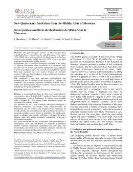
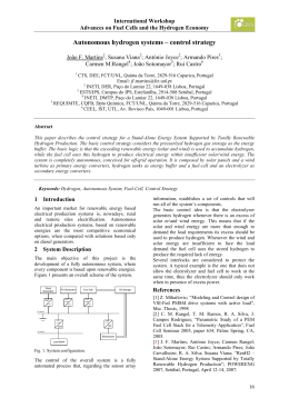
Figure 1 shows the evolution of fossil energy’s share of income as well
as the fossil-fuel price. As can be seen, fossil energy’s share of income is
highly correlated with its price and it is not constant. Specifically, the share
starts out around three percent in 1949 and then decreases somewhat up
to the first oil price shock when it increases dramatically. The share then
4
The GDP data is taken from the Bureau of Economic Analysis at
http://www.bea.gov/histdata/Releases/GDP and PI/2009/Q4/Third March-262010/Section1ALL xls.xls. For the USEIA reference, see tables 1.3 and 3.1, respectively,
available at http://www.eia.gov/totalenergy/data/annual/. The Net export of fossil fuel
is taken from the Annual Energy Review 2011, Table 3.9.
5
Since housing services is included in GDP, we include fossil fuel used for heating residential houses in E. Including the use of petroleum consumption for passenger cars but not the output of private transportation services would likely bias our
results since the short-run demand for fossil fuel for private transportation is fairly
elastic (see Kilian, 2008). The data on petroleum consumption is taken from the Federal Highway Administration, Highway Statistics Summary to 1995, table VM-201a at
http://www.fhwa.dot.gov/ohim/summary95/section5.html.
8
falls drastically between 1981 and the second half of the nineties and then
finally increases again. The share does not seem to have an obvious longrun trend, implying that the possibility that the unitary elasticity is a good
approximation for the very long run cannot be excluded. For the medium
term, however, the data seems hard to square at least with an exact CobbDouglas production function.
The Factor Share of Energy in the U.S. Economy
0.06
0.04
0.02
0
1940
1950
1960
1970
1980
1990
2000
2010
2000
2010
Fossil Fuel Price (composite)
4
3
2
1
0
1940
1950
1960
1970
1980
1990
Figure 1. Fossil energy share and its price
B.
A nested CES production function
A slightly broader class of production functions is offered by the following
nested CES production function:
9
(2)
ε
i ε−1
h
E ε−1
ε−1
ε
ε
+
γ
A
E
,
Yt = (1 − γ) At Ktα L1−α
t
t
t
where L is labor, A capital/labor-augmenting technology, AE fossil energyaugmenting technology and ε the elasticity of substitution between capital/labor and fossil energy. γ is a share parameter. It should be pointed
out, however, that the specific nesting of capital, labor and energy in (2) is
not important for our results. In fact, all the results below still hold with
alternative specifications where the elasticity of substitution between capital
and energy is allowed to differ from the elasticity of substitution between
labor and energy.6
The first argument in the production function is a Cobb-Douglas composite of capital and labor, ensuring that the relative shares of capital and labor
inherits their properties from the usual Cobb-Douglas form used in growth
studies. The second argument, again, is energy. Note that when ε = ∞,
the Cobb-Douglas composite and fossil energy are perfect substitutes, when
ε = 1, the production function collapses to being Cobb-Douglas in all input arguments; and when ε = 0 the Cobb-Douglas composite and energy
are perfect complements, implying a Leontief function in the capital-labor
composite and energy.
Note also that this nested CES function implies that there are two distinct factor-augmenting technical change series. Equation (2) can thus be
6
similar with the alternative specification Yt =
h All the results are, for instance,
ε α
i ε−1
ε−1
E ε−1
ε
L1−α
. This specification requires annual data
(1 − γ) [At Kt ] ε + γ At Et
t
on capital’s share of output, which we compute as rt Kt /Qt = 1 − Wt Lt /Qt − Pt Et /Qt .
The data used to compute the wage share is taken from the Bureau of Economic Analysis,
and it includes data on self-employment income.
10
used to identify the evolution of the two technology trends A and AE : A
is capital/labor-saving and one is energy-saving. In the next section, we
will formally estimate these trends along with the key elasticity parameter
ε. However, let us first start with how one could use a procedure similar to
that in Solow (1957), provided one knew the correct production function. In
his seminal paper, Solow shows how to measure technology residuals with a
general production function with two key assumptions: perfect competition
and constant returns to scale. To measure factor-specific technology residuals, which we aim for here, one needs to make more assumptions on the
production function.7 Specifically, we assume that the production function
takes the form given by (2).
For the estimation below, we impose α = 0.3, as we know that it will fit
the data on the relative capital/labor shares well. The elasticity parameter
ε will be estimated, but for now assume that we knew its value, along with
γ.
Under perfect competition in input markets, marginal products equal factor prices, so that labor’s and energy’s shares of income are respectively
given by
(3)
LShare
t
At Ktα Lt1−α
≡ (1 − α) (1 − γ)
Qt
ε−1
ε
and
(4)
EtShare
AE
t Et
≡γ
Qt
ε−1
ε
.
7
This strategy has been used in many applications; see, e.g., Krusell et al. (2000) and
Caselli and Coleman (2006).
11
Equations (3) and (4) can be rearranged and solved directly for the two
technology trends At and AE
t . This delivers
(5)
ε
ε−1
Qt
LShare
t
At = α 1−α
(1 − α) (1 − γ)
Kt Lt
and
(6)
AE
t
ε
Qt EtShare ε−1
=
.
Et
γ
Note that with ε and γ given, and with data on Qt , Kt , Lt , Et , LShare
and
t
EtShare , equations (3) and (4) give explicit expressions for the evolution of
the two technologies. Clearly, the parameter γ is a mere shifter of these
time series and will not play a role in the subsequent analysis. The key
parameter, of course, is ε.
The goal of the exercises to follow is to gauge what a reasonable value of
ε is, then to use equations (5) and (6), and finally to study the properties of
these two implied time series: what their trends are and, more importantly,
how they co-vary and relate to the energy price.
III.
Estimation
We now estimate the elasticity ε, together with some other parameters,
directly with a maximum-likelihood approach. The idea behind the estimation is perhaps simplistic but, we think, informative for our purposes: we
specify that the technology series are exogenous processes of a certain form
and then estimate the associated parameters along with ε. The technology
processes have innovation terms and the maximum likelihood procedure, of
course, chooses these to be small. Hence, the key assumption behind the es-
12
timation is to find a value of ε such that the implied technology series behave
smoothly, or as smoothly as the data allows. This may not be appropriate
for other kinds of series but it seems reasonable precisely to require that
changes in technology are not abrupt.
As for the particular specification of our technology processes, we also
choose parsimony: we require that they be stationary in first differences
and have iid, but correlated, errors. Other formulations, allowing moving
trends or serially correlated errors, will undoubtedly change the details of the
estimates we obtain, but they are unlikely to change the broad findings. As
a support for this position, and after showing the results of the estimation,
we will discuss implications of radically different values for ε: why they
produce series for technology that are not smooth at all.
A.
The technology processes
Our formulation is

(7)

at
aE
t


−
at−1
aE
t−1


=
θ
A
θE


+

E

where at = log(At ), aE
t = log(At ) and $ t ≡
$A
t
$E
t
$A
t
$E
t

,

 ∼ N (0, Σ).
Dividing equations (5) and (6) by their counterparts in period t − 1 gives
(8)
ε
Share ε−1
α
L1−α
Qt Kt−1
Lt
At
t−1
= α 1−α
At−1
Qt−1
LShare
Kt Lt
t−1
13
and
ε
Qt Et−1 EtShare ε−1
AE
t
=
.
Share
Et Qt−1 Et−1
AE
t−1
(9)
Taking logs of (8) and (9) and using (7) in these expressions gives allows
us to write the system as
st = θ −
(10)
ε
zt + $ t ,
ε−1
where

st ≡ 
log
Qt
Ktα L1−α
t
log
Qt
Et
− log
− log
Qt−1
α L1−α
Kt−1
t−1
Qt−1
Et−1



and zt ≡ 
log LShare
t
−
log LShare
t−1
Share
log EtShare − log Et−1
The log-likelihood function is now given by
(11)
− N2 log |Σ| −
1
2
N
P
t=1
l (s|θ,ε, Σ) =
T −1
ε
st − θ − ε−1
zt
Σ
st − θ −
ε
z
ε−1 t
+ const.
B.
Results
Maximization of (11) with respect to θ, ε, and Σ gives the estimated
parameters straightforwardly. The data for output, energy, and its price
was discussed above. Data on the labor force is taken from the Bureau
of Labor Statistics, whereas data on the capital stock as well as the data
required to compute labor’s share of income are taken from the Bureau of

.
14
Economic Analysis.8
The results of our estimation are displayed in Table 1.
Table 1—Estimated parameters
θA
0.0132
(0.0021)
θE
0.0136
(0.0030)
ε
0.0044
(0.0127)
Standard errors in parenthesis
There are two noteworthy features here. One is that the technology trends
are both positive and of very similar, and a priori reasonable, magnitude.
The second, and more important, point is that the elasticity of substitution
between the capital/labor composite and energy is very close to, and in fact
not significantly different from, zero. Thus, the CES function that fits the
annual data on shares best—where we again emphasize that the estimation procedure penalizes implied technology series that are not smooth—is
essentially a Leontief function.
Turning to the estimated covariance matrix, it is given by

Σ = 10−3 ∗ 
0.28
−0.03
−0.03
0.48

.
Thus, the energy-saving shocks are somewhat more volatile than are capital/laborsaving technology shocks, and the two shocks are somewhat negatively correlated in the annual data.
8
We use online data from the BLS on the labor force. The data is available at http://www.bls.gov/webapps/legacy/cpsatab1.htm#a1.f.1.
For the capital
stock, we use online-data on the net stock of private non-residential fixed assets
available at http://www.bea.gov/histdata/Releases/FA/2009/AnnualUpdate August-172010/Section4ALL xls.xls (table 4.2). Labor’s share of income is calculated as (compensation of employees / (compensation of employees + private surplus - proprietors’ income)
) and is taken from BEA, National Accounts 2008:Q1, table 11100.
15
What features of the data make our estimation select a value for ε close
to 0? As a way of interpretation and before looking at implications of our
estimates, we first examine how higher values for the elasticity would change
the implied technology series. We then return to our estimates.
C.
A high elasticity of substitution
The Cobb-Douglas function, with its unitary elasticity, does not allow the
two technology series to be separately identified. For any non-unitary value,
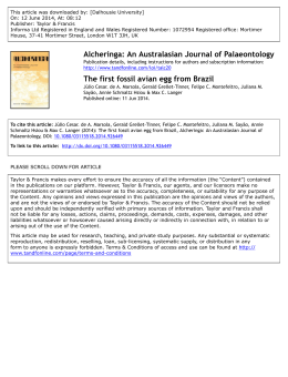
however, this is possible. We thus set ε = 0.8. The evolution of the implied
fossil energy-saving technology is presented in Figure 2. Clearly, the series
implied by a high ε is a rather nonsensical one if interpreted as technology.
It features large jumps and dives; it increases by more than 50,000 percent
between 1980 and 1998 and decreases by more than 7,600 percent between
1998 and 2009.
35
30
25
20
15
10
5
•←The first oil shock
0
1940
1950
1960
1970
1980
1990
2000
2010
Figure 2. Energy-saving technology with an elasticity of 0.8
16
To understand this result, take the first oil shock as an example. The price
increase in 1973 would then, with a fairly high elasticity, call for much lower
energy consumption in U.S. business. However, this fall in consumption is
not observed in the data. According to the model, this must then be because
of a huge fall in the energy-specific technology value: oil is now much more
expensive, but it is also less efficient in producing energy services, the net
result of which is a rather constant level of oil use. Similarly, when the price
falls in the nineties, an increased demand for energy is expected, but again,
this does not take place in the data. The reason, from the perspective of
the model, must be that the energy-specific technology increases sharply—
by 350 percent in just one year. The mean annual growth rate in AE during
the period with the chosen elasticity is negative (-1.42 percent) and the
standard deviation is very high (62.8 percent).9
When thinking about the implications of the price movements for fossil
fuel, note that the exact reason for the large volatility of fossil fuel prices is
not important. This is key since there are two very different, and contrasting, interpretations of the large movements in oil prices. Barsky & Kilian
(2004), in particular, argue that the conventional view, i.e., that events in
the Middle East and changes in OPEC policy are the key drivers of oilprice changes, is incorrect. Rather, they contend, the price changes were
engineered by U.S. administrative changes in price management. Be that
as it may, what is important here is simply that firms actually faced the
prices we use in our analysis. In conclusion, at least from the perspective
of the assumptions of the theory, it is not possible to maintain as high an
elasticity of substitution between capital/labor and energy as 0.8. In fact,
9
The capital/labor-augmenting technology is highly volatile too when ε is high, but
the effects of high substitutability are larger on the energy-saving technology.
17
it takes much smaller εs to make the volatile, non-technology-like features
go away—only values below ε ∼ 0.05 make the series settle down. We now
turn to what those series look like for the near-Leontief case.
D.
Low elasticity: implications
The near-Leontief case, i.e., ε close to zero is rather robust in that once
the substitution elasticity is in this low range, the features of the technology
series do not vary noticeably. So consider now instead a low elasticity and set
ε = 0.02, a value slightly higher than the estimated one, but yielding almost
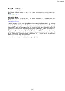
identical output. The implied energy-saving technology trend is presented
in Figure 3. The figure shows the path for fossil energy-saving technology
AE . As is evident, we observe a smooth, increasing, and overall reasonablelooking graph for fossil energy-specific technology. The mean growth rate is
1.49 percent and the standard deviation is 2.37 percent.10
The figure also shows separate trends lines before and after the first oilprice shocks: 1949–1973 and 1973–2009. Clearly, the technology series appears to have a kink around the time of the first oil price shock. In fact,
the growth rate is 0.15 percent per year up to 1973 and 2.44 percent per
year after 1973. The fact that the kink occurs at the time of the first oil
price shock suggests that the higher growth rate in the technology is an
endogenous response to the higher oil price.
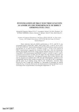
Figure 4 displays both the fossil energy-saving technology and the oil price
and suggests that the energy-saving technology seems to respond to price
changes at even higher frequencies. The figure specifically shows that from
1949 up the first oil shock in 1973, the price decreases and at the same time,
10
The energy-saving technology does not change much for elasticities in the interval
(0, 0.05).
18
2.6
2.4
AE
Regression lines
2.2
2
1.8
1.6
1.4
1.2
•←The first oil shock
1
0.8
1940
1950
1960
1970
1980
1990
2000
2010
Figure 3. Energy-saving technology with an elasticity of 0.02
the energy-specific technology grows only slowly at a rate of 0.15 percent
per year. After the large price increase in 1973, the technology grows at
the significantly higher rate of 3.69 percent/year up to 1981. However, as
the price starts decreasing between 1982 and 1998, the growth rate in the
energy-saving technology also slows down to 1.80 percent/year. The price
then increases from around 1996 up to 2009 and the growth rate in the
technology increases to a rate of 2.35 percent/year. In the last period of our
data, the fossil fuel price decreases significantly. If the relation is robust,
this can be expected to have a negative effect on the growth in energy-saving
technology.
What does a low elasticity imply for the evolution of the capital/laboraugmenting technology? The series for A is plotted the solid line in Figure
5, alongside the AE series. A too is smooth and increasing graph and very
much looks like the conventional total-factor productivity (TFP) series. The
19
4.5
4
AE
Real fossil fuel price
3.5
3
2.5
2
1.5
1
0.5
1940
1950
1960
1970
1980
1990
2000
2010
Figure 4. Energy-saving technology and the energy price compared
mean growth rate in A is 1.31 percent and the standard deviation is 1.68
percent. When we compare it to the AE series, we see that the two series
nearly mirror each other.11 In the beginning of the period, the capital/laboraugmenting technology series grows at a relatively fast rate, whereas the
growth rate for the energy-augmenting technology is relatively slow. This
goes on until around 1970, i.e., somewhat just before the first oil price shock.
After 1970, the energy-augmenting technology grows at a faster rate and the
growth rate for the capital/labor-augmenting technology slows down. This
continues up to the mid-1980s. Hence, the much-discussed productivity
slowdown coincides with a faster growth in the energy-saving technology.
Our impressions that there is a medium-run negative correlation between
the two technology series are formalized by applying an HP filter to the two
series, taking out the cyclical component, and regressing the trend growth
11
Both series have been normalized so that the initial value is 1.
20
2.6
A
2.4
AE
2.2
2
1.8
1.6
1.4
1.2
1
0.8
1940
1950
1960
1970
1980
1990
2000
2010
Figure 5. Energy- and capital/labor-saving technologies compared
of energy-augmenting technology gAE , on the trend growth of the capitalaugmenting technology gA .12 We find the relation
(12)
gAE = 2.26 − 1.23gA ,
which is significant at the 1% level. This result can be compared with Popp
(2003), who uses expenditure on energy R&D and non-energy R&D and
finds a correlation coefficient of -0.41.
At this point, let us take stock of what we have found. Rather simple,
though in our view revealing, features of the share and the price data are
suggestive of (i) an aggregate CES technology in a capital/labor composite
and energy that is close to Leontief on an annual horizon and (ii) of implied
movements in factor-saving technologies that are negatively correlated. To
12
λ is set to 100 which is standard for annual data.
21
us, this points in the direction of a model of directed technical change. In
the least complex fashion of illustrating this, one envisions a fixed R&D
resource that can be allocated between two sectors, and where allocating a
larger share to one sector implies a faster growth rate in that sector, as a
result of which the other sector’s growth rate will deteriorate. Of course,
this interpretation also indicates that there are substantial costs associated
with improving energy efficiency, since a higher energy efficiency will come
at the cost of lower growth of capital/labor-efficiency. In order to explore
this mechanism, in the next section we construct a formal model of directed
technical change. This model can be thought of as a putty-clay model in
which the substitution possibilities between capital/labor and energy are
fixed ex post but chosen (optimally, or otherwise) ex ante.
IV.
A model of directed technical change
The previous sections suggest that energy saving and capital/labor saving,
captured as shift parameters in an aggregate production function, respond
to incentives. In this section, we formalize that idea, allowing us to fully
work out the logic of directed technical change. One of the implications of
the analysis, as we shall see, is that the long run will feature a constant
energy share, thus giving a much higher long-run elasticity between energy
and capital/labor. We also use the model to carry out quantitative exercises
that rely on the empirical relationships—in particular the negative mediumrun correlation between the growth in energy-saving and in capital/laborsaving—obtained in the first section of our paper.
Our analysis of directed technical change allows us to address two additional issues. One of these regards “peak oil”. Clearly, oil use has increased
22
over time and since it is in finite supply it must peak at some point and
then fall. The issue here is that standard models do not predict a peakoil pattern: they predict falling oil use from the beginning of time. By
standard models, here, we refer to settings relying on the classic work on
nonrenewable resources in Dasgupta and Heal (1974) and with high substitutability between oil and capital/labor. A simple case makes the point:
with standard preferences (logarithmic utility, discounted in a standard way
over time), Cobb-Douglas production, and full depreciation of capital between periods, along with the assumption that oil is costless to extract, oil
use will fall at the rate of utility discount. Our perspective on this result,
which is robust to moderate changes in all the assumptions, is that a much
lower elasticity between oil and capital/labor may allow a peak oil result, a
possibility we examine after laying out the model.
A second issue we address with the model, given its constant long-run
share of energy costs, is just how large this share will be quantitatively.
Our benchmark model assumes that energy only comes from oil. This case
is easily analyzed and interesting, despite its unrealistic nature, since it
makes the “need for alternative energy sources” rather clear: the oil share
must, under reasonable parameterizations of the model, rise over time and
eventually become quite high. This oil-only case then naturally leads into a
second case, that with either a more abundant fossil-fuel source (say, coal)
or an alternative, non-fossil energy source, and we conclude by showing that
such a model predicts a more modest long-run share for energy costs.
23
A.
The setting
In order to keep the model simple and transparent, we assume log utility, literal Leontief production, full depreciation, and zero-cost fossil-fuel
extraction. These assumptions are not that unreasonable if the time period
is 10 years and the time horizon is not too long. We focus on the planning
solution and sidestep any issues coming from suboptimal policy with regard
to R&D externalities, monopoly power due to patents as well as the market
power in the energy sector. We also ignore the (global) climate externality,
which might still be of concern in this context even though the damages
to the U.S. economy have been estimated to be small. Clearly, these are
important issues and we are studying them in related work, but we believe
that they are not of primary concern for our main points here.13
The representative consumer thus derives utility from a discounted sum of
the logarithms of consumption at different dates. This is also the objective
function of the planner, i.e.,
∞
X
β t log Ct .
t=0
The period resource constraint is
Ct + Kt+1 = min At Ktα L1−α
, AE
t
t Et ,
where the right-hand side specifies a Leontief production function. The
13
See Nordhaus and Boyer (2000) and Golosov et al. (2012).
24
growth rates of the technology trends are assumed given by
(13)
(14)
At+1
≡ 1 + gA,t = f (nt )
At
AE
t+1
≡ 1 + gAE ,t = f E (1 − nt ),
AE
t
where we interpret n as the share of a fixed amount of R&D resources that
is allocated to enhancing the efficiency of the capital/labor bundle. The
functions f and f E are increasing. Of course, an increase in A (AE ) is
equivalent to a decrease in the Leontief input requirement coefficient for the
capital/labor (energy) bundle. By changing n, the planner can direct technical change to either of the two. When A grows at a different rate than AE ,
the requirement of energy relative to the requirement of the capital/labor
bundle changes. Thus, factor substitutability exists in the long run. Finally,
we assume that energy comes from a fossil-fuel source satisfying
Rt+1 = Rt − Et ∈ [0, Rt ],
where Rt is the remaining stock of oil in ground. We also restrict labor
supply so that lt = 1 for all t. This can be thought of as “full employment”.
We let k denote capital henceforth, as in capital per unit of labor.
B.
Planning problem
We focus on interior solutions such that capital is fully utilized. This
requires initial conditions where capital is not too large, in which case it
could be optimal to let some capital be idle for some time. In a deterministic model with full depreciation and forward-looking behavior, less than
25
full utilization can only occur in the first period.14 Due to solutions being
interior, we replace the Leontief production function by the equality
At ktα = AE
t Et
(15)
and let the planner maximize
max
∞
X
β t log(At ktα − kt+1 ).
t=0
Condition (15) will be referred to as the “Leontief condition”. In addition,
the planner must respect the constraints
∞
X
(16)
Et ≤ R0 ,
t=0
and (13)–(14).
Let the multipliers on the constraints be β t λt on the Leontief condition
(15), κ on the resource constraint (16) and β t µt , and β t µE
t , respectively for
the two R&D constraints (13)–(14). The first-order conditions are: for kt+1 ,
the Euler equation
(17)
1
=β
(1 − st )At ktα
1
α−1
− λt+1 αAt+1 kt+1
;
α
(1 − st+1 )At+1 kt+1
for Et ,
β t λt AE
t = κ;
14
In a model with stochastic shocks, we could have reoccurring periods of less than
full capital utilization.
26
for At+1 and AE
t+1 , respectively,
µt = β
1
α
− λt+1 kt+1 + µt+1 f (nt+1 )
α
(1 − st+1 )At+1 kt+1
and
E
E
µE
t = β λt+1 Et+1 + µt+1 f (1 − nt+1 ) ;
and, for nt ,
E
E 0
µt At f 0 (nt ) = µE
t At (f ) (1 − nt ).
Here, st is the saving rate out of output. Of course, in a recursive formulation, optimal savings depend on the vector of state variables. Here, we
solve the model sequentially and present the solution as a time series.
Solving For Saving Rates Conditional On Energy Use
The second first-order condition above can be used to solve for λt in a
useful way:
λt = κ
1
Êt ,
At ktα
where we have defined Êt ≡ β −t Et . If this expression is inserted into the
Euler equation we obtain
(18)
st
= αβ
1 − st
1
− κÊt+1 .
1 − st+1
Using ŝt ≡ st /(1 − st ) and the algebraic identity
1
1−s
rewrite this equation as
ŝt = αβ 1 + ŝt+1 − κÊt+1 .
= 1+
s
,
1−s
we can
27
Solving this forward yields
∞
X
αβ
−κ
ŝt =
(αβ)k+1 Êt+k+1 .
1 − αβ
k=0
(19)
Thus, given a sequence {Êt } and a value of κ, this equation uniquely, and
in closed form, delivers the full sequence of savings rates. We can see from
this equation that the more energy is used in the future (in relative terms),
the lower is current ŝ, implying a lower current saving rate. The intuitive
reason for this is that more capital requires more fossil fuel and/or more
energy efficiency. This limits the value of accumulating capital and more
so, the more scarce is fossil fuel. If fossil fuel were not scarce, κ = 0 and
αβ
1−αβ
ŝ =
⇒s = αβ since the model in this case collapses to the textbook
Solow model.
Solving For Energy Use And R&D
From the original Euler equation, we have that
β
1
1
kt+1
st
α
− λt+1 kt+1
=
=
.
α
α
(1 − st+1 )At+1 kt+1
αAt+1 (1 − st )At kt
α(1 − st )At+1
Inserted into the first-order condition above for At+1 , we obtain
µt =
st
+ βµt+1 f (nt+1 ).
α(1 − st )At+1
Multiplying this equation by At+1 and defining µ̂t ≡ µt At+1 , we obtain
(20)
µ̂t =
st
ŝt
+ β µ̂t+1 = + β µ̂t+1 .
α(1 − st )
α
Given a sequence of saving rates, this equation can be solved for the µ̂t
28
sequence. Iterating forward on (20) is also a discounted sum; it delivers
∞
1X k
β ŝt+k .
µ̂t =
α k=0
Recalling that µ̂t is the current marginal value of capital-augmenting technology, it is intuitive that the more is saved into the future, the higher is
the value of µ̂t . Using equation (19), we can write this directly in terms of
the Ê sequence. By direct substitution and slight simplification we obtain
∞
(21)
∞
κ X kX
β
β
(αβ)j+1 Êt+1+k+j .
µ̂t =
−
(1 − β)(1 − αβ) α k=0
j=0
Similarly, from the expression for λt above, we can write
λt+1 Et+1 = κ
Et+1
Êt+1
Êt+1 = κ E ,
α
At+1 kt+1
At+1
where the last equality follows from the Leontief assumption. Inserted into
the first-order condition for AE
t+1 , we obtain
#
Ê
t+1
+ µE,t+1 f E (1 − nt+1 ) .
µE
t = β κ E
At+1
"
E
E E
Multiplying this equation by AE
t+1 and defining µ̂t ≡ µt At+1 , we obtain
h
i
E
µ̂E
=
β
κ
Ê
+
µ̂
t+1
t
t+1 .
Given a sequence of normalized fossil fuel uses, this equation can be solved
29
for the µ̂E
t sequence. It can also be solved forward:
µ̂E
t
(22)
=κ
∞
X
β k+1 Êt+k+1 .
k=0
In parallel to the case of capital-augmenting technology, the more energy
is used in the future and the larger is fossil fuel scarcity, the higher is the
marginal value of energy-enhancing technology.
Finally, rewriting the first-order condition for nt above in terms of the
redefined multipliers, we arrive at
µ̂t
f 0 (nt )
(f E )0 (1 − nt )
= µ̂E
.
t
f (nt )
f E (1 − nt )
From this equation we can solve for nt uniquely for all t, given the values
of the multipliers, so long as f is (strictly) increasing and (strictly) concave
(either the monotonicity or the concavity need to be strict). Using the
expressions above for the multipliers, we obtain
(23)
(f E )0 (1 − nt )f (nt )
=
f E (1 − nt )f 0 (nt )
β
κ(1−β)(1−αβ)
−
k P∞
j+1
Êt+1+k+j
k=0 β
j=0 (αβ)
.
P∞ k+1
Êt+k+1
k=0 β
1
α
P∞
This equation enables us to solve for nt directly as a function of the future
values of Ê. The more energy is used in the future, the lower is current n, i.e.,
the more R&D labor is allocated to energy-saving now. It is straightforward
to solve this equation numerically for transition dynamics. However, one can
characterize long-run growth features more exactly.
30
C.
Balanced growth
On a balanced path, the saving rate is constant and so, from the Euler
equation, Êt is constant. Recalling the definition Êt ≡ β −t Et , this means
that Et = (1 − β)Rt and Rt = β t R0 implying Ê = (1 − β)R0 . The saving
rate st the balanced growth path is constant and ŝt =
st
1−st
=
αβ(1−κÊ)
.
1−αβ
The Leontief condition holds for all t when E falls at rate β, so that
At+1
At
kt+1
kt
α
AE
β,
= t+1
AE
t
implying (since nt has to be constant)
f (n)
α
kt+1
= f E (1 − n)β.
ktα
A constant saving rate implies, if k is to grow at a constant rate, that k
1
grows at the gross rate f (n) 1−α . Thus, we have
α
f (n)f (n) 1−α = f E (1 − n)β
or
(24)
1
f E (1 − n) = β −1 f (n) 1−α .
This equation, on the one hand, describes a positive relation between
1
the growth rates of A and AE : 1 + gAE = β(1 + gA ) 1−α . The positive
relation comes from the two inputs growing hand-in-hand due to the shortrun substitution elasticity between capital/labor and oil being zero. On the
other hand, equation (24) allows us to solve for n, and therefore the point
31
on the positively-sloped curve, which in turn implies a long-run growth rate
of consumption for the economy. This, however, requires a specification and
calibration of f E and f . We will carry out a calibration below.
The solution for n can be used in equation (23) to solve for the steady-state
value for κ. Using the finding that Ê is constant, (23) becomes
1 − κÊ
(f E )0 (1 − n)f (n)
=
.
E
0
f (1 − n)f (n)
κÊ(1 − αβ)
(25)
Thus, given the n from equation (23), we obtain κÊ from equation (25). We
then also obtain the saving rate, as specified above, since it depends on κÊ.
Notice that since κÊ is pinned down independently of initial conditions and
Ê = (1 − β)R0 , any increase in R0 just lowers the κ by the same percentage
amount on a balanced growth path. Of course, a balanced path from time
0 also requires that the initial vector (k0 , A0 , AE
0 , R0 ) satisfy
A0 k0α = AE
0 (1 − β)R0 ;
if and only if this equation is met will the economy grow in a balanced way
all through time.
Let us finally find the energy share and the value of the fossil fuel resource
in balanced growth. This is straightforward to derive using the fact that
the current shadow price of the energy resource is β −t κ. Dividing by the
marginal utility of consumption to get a price in consumption units and
multiplying by
Et
Yt
gives the energy share;
κ
EtShare
β −t κ Et
u0 (c )
= 0
= β −t Et
u (ct ) Yt
At
32
and since u0 (ct ) =
1
,
(1−s)AE
t Et
this is
E Share = κ (1 − s) Ê.
Using this in the Euler equation (18) along a balanced growth path yields
s = αβ 1 − (1 − s) κÊ
= αβ 1 − E Share .
Thus,
E Share
1−s
= κÊ and αβ =
s
.
1−E Share
Using (25), we obtain
(f E )0 (1 − n)f (n)
1 − E Share
=
,
f E (1 − n)f 0 (n)
E Share
(26)
which delivers the energy share as a function of n. The steady-state income
share of energy is thus fully determined by technological constraints implied
by the R&D functions. In particular, it does not depend on the amount of
oil left in the ground (but does rely on oil use going to zero asymptotically
at rate β).15
D.
Calibration and long-run predictions
To obtain a long-run value for n, we need information on f and f E , according to equation (23). The natural restrictions to place on these functions are
in the past data, as described above. In particular, we observed a negative
medium-run correlation between the growth rates of A and AE variables
and, more precisely, the regression equation (12) details not only the rela15
Utility functions with different curvature yield oil use going to zero at a different
rate. Our calculations, however, show the departures from logarithmic utility to have
relatively minor effects on this rate and on the long-run oil share.
33
tion between the two growth rates but also an intercept. In fact, as we shall
show, for our main questions in this section we do not need to go beyond
this information and find specific functional forms for f and f E .
So first jointly consider the positive relation (24) between gA and gAE
and the negative one (12) given by our data; these are depicted in Figure 6
below. The upward-sloping line (24) is drawn for α = 0.3 and β = 0.9910 —
these are relatively standard values in the growth literature. The estimated
downward-sloping line (12), intuitively, is informative of the functions f and
f E : the growth rates gA and gAE in our theory are related through equations
(13)–(14), which imply
1 + gAE = f E (1 − f −1 (1 + gA )).
(27)
Our linear regression can be thought of as a linearization of equation (27).
Using the linearization, we can immediately use the graph for predicting
the long-run values of the two growth rates, since these will simply be given
by the intersection of the two lines in the figure. We see that the curves
intersect at gA = 0.0074 and gAE = 0.021 implying a long-run growth rate
of consumption of 1.07% per year. That is, our theory implies that despite
oil running out, consumption will grow in the long run, albeit at a relatively
modest rate.
Let us finally determine the long-run value of the oil share of output.
Equation (27) can be differentiated to obtain
−
(f E )0 (1 − n)f (n)
1 − E Share
dgAE
= E
=
.
dgAE
f (1 − n)f 0 (n)
E Share
Now notice that this expression coincides with the left-hand side of equation
34
0.04
0.035
0.03
gAE
0.025
0.02
0.015
0.01
0.005
0
0
0.002 0.004 0.006 0.008
0.01
gA
0.012 0.014 0.016 0.018
0.02
Figure 6. Quantitative determination of the long-run growth rates
(26), whose right-hand side equals (1 − E Share )/E S hare. Hence, this being
a steady-state relation, the steady-state income share of energy can be determined if we use the linearization above. The regression coefficient of gAE
on gA (the slope in Figure 6) was found to be -1.23, implying a long-run
fossil-fuel income share of 45%. This is a large number, in fact so large that
it would be hard to imagine that significant resources would not be spent
on developing alternative sources of energy. For this reason, we look at such
a possibility below. However, one might wonder whether the value around
40% we obtain is robust. As noted above, this share is only determined by
the shape of the f and f E functions, and to obtain an income share more
in line with historically observed values, we need a much higher slope than
-1.23: it would have to be around -20, i.e., one unit less of growth in A
would deliver 20 units more of growth in gAE . This is only possible if our
estimate based on historical data is off by more than an order of magnitude.
35
E.
Peak oil?
In this section the aim is to calculate the transition path for our economy.
If the initial value of A (relative to AE ) is low enough, the idea is then
that the economy would mainly accumulate A initially, with an accompanying increase in E: a peak-oil pattern. To use the model for quantitative
predictions, we specify the R&D functions to be
(28)
f (nt ) = Bnφt ,
f E (1 − nt ) = BE (1 − nt )φ .
Inverting the first function, substituting, and taking logs yields
1 + gAE = ln BE + φ ln 1 − e
1+gA −ln B
φ
The three parameters of these functions are calibrated using the relation
between the two technological growth rates found in the first part of the
paper. Specifically, we use the average growth rates of the two technology
series for the pre-oil crisis (1946–73), the oil crisis (1974–84), and the postoil crisis (1985–2009). These six observations allow us to identify the three
parameters of the R&D functions and the three unobserved values of n. In
addition we use α = 0.3 and β = 0.9910 .
The model is easily solved numerically. We find that if A0 and k0 are set
to 45 and 55 percent of their balanced-growth values, respectively, we obtain
five decades of increasing fossil fuel use. During the transition, E has to grow
fast to keep up with the quickly increasing capital and capital/labor-saving
technology growth. The results are plotted in Figure 7 below.
34
36
THE AMERICAN ECONOMIC REVIEW
Annual net growth rate of E (%)
2
Annual net growth rates of technologies (%)
3
1
2
0
1
-1
0
5
10
15
20
0
A
AE
0
5
0.4
1.5
0.3
1
0.2
0.5
0.1
0
5
10
15
20
10
15
20
15
20
Eshare
Annual net growth rate of K (%)
2
0
MONTH YEAR
0
0
5
10
Figure
7. Transition
Figure 6. Transition paths in the
model
with directed energy saving technichal change. Initial values for 0 and 0 are respectively 45 and 55
percent of the balanced growth value.
F. An alternative energy source
Our setting above relies on oil being the only source of energy. Today,
saving, and
another which saves on capital and labor. Within this framework
oil accounts for a little less than half U.S. energy supply. However, the
we then first
formally
estimate
elasticity
of substitution
amount
of oil remaining
in the
the ground
is rather
limited, at leastbetween
compared energy
to the amount
available
coal.
can also
expect the emergence of energyand capital/labor
andof find
it to
beWe
close
to zero.
efficient non-fossil alternatives, especially given our estimates above of a very
Second, we find that the fossil energy-saving technology appears to rehigh long-run oil share of output. In this section, we consider an alternative
spond to to
economic
incentives.
Specifically,
thefrom
growth
rate of
this
technoloil. To simplify
the analysis,
we abstract
oil entirely.
The
main
purpose
of the
section
is to assess what
the percent/year
long-run value ofafter
the energy
ogy increased
from
0.65
percent/year
to 2.24
the first oil
share will be in this alternative setting.
price shock
in 1973. The measured rise in the growth rate thus seems to be
Our modeling of the alternative energy source—we will refer to it as “coal”
a response to the oil-price shocks. A closer look at the correlation between
but it could equivalently be thought of as a non-fossil resource—is simply
the growth rate of the technology and the price shows that whenever the
to assume that labor used in final production could alternatively be used
price of fossil fuel stays relatively high for a period of time, the technology
grows at a faster rate and vice versa.
Third, the two technology series display a negative medium-run correlation. When one technology grows relatively faster the growth rate of the
37
in the production of an energy source, again denoted E, with at a constant
marginal cost per unit of coal. Thus, E = ξl, where l is the amount of labor
used in energy production and 1 − l is used in the production of the final
good. Output is then given as follows:
ct + kt+1 = min At ktα (1 − lt )1−α , AE
t ξlt .
Note the contrast with oil: coal is costly to extract, whereas we considered
oil not to be. This is a rough approximation but captures a key aspect
of these energy sources: the largest part of the market price for oil is a
Hotelling rent rather than a production cost, whereas the reverse is true for
coal.16
It is straightforward to solve the coal model along the same lines as in
Sections IV.B–IV.C. We refer the interested reader to an online appendix
for the details. A key property of the model for the present purposes is that
t
t
/(1 + (1 − α) 1−l
).17
the oil share will simply equal wt lt /yt = (1 − α) 1−l
lt
lt
On a balanced path, lt will converge, and its solution will depend on the
parameters of the research technologies. Here, we will assume that the R&D
technology for advancing coal-saving is the same as that for oil, so that the
tradeoff between coal-saving and capital/labor-saving again can be measured
by the downward-sloping line in Figure 6. With the parameter values used
in that context, we obtain a long-run energy share of 29%, which is less
than for oil but still large. Along with this share, we found the growth of
16
See Hotelling (1931). Clearly, the correspondence here between the physical classification of fossil fuel into oil and coal and the economic distinction is not perfect. In
particular, some sources of non-conventional oil have extraction costs that are large relative to their price. Such oil is, in economic terms, to be considered equivalent to coal.
1−α
17
This can be derived from the firm’s problem, which involves maximizing At ktα l1t
−
α 1−α
E
wt (l1t + l2t ) subject At kt l1t = ξAt l2t .
38
A to be 1.3% and that of AE to be 1.9%, resulting in consumption growth
of 1.9%. Clearly, a fuller model of energy supply would include several
energy sources simultaneously and gradual phasing out of oil/phasing in of
alternatives. However, the long-run features of such a model would likely
not differ markedly from those examined in this section.
V.
Concluding remarks
In this paper we have estimated an aggregate production function on historical U.S. data in order to shed light on how the economy has dealt with
the scarcity of fossil fuel. The evidence we find strongly suggests that the
economy directs its efforts at input-saving so as to economize on expensive,
or scarce, inputs. We also used this evidence to inform estimates of R&D
technologies, allowing us to make some projections into the future regarding
energy use and, ultimately, consumption growth. Our analysis is quite stylized but we believe that it captures both qualitatively and quantitatively
important aspects of energy resource scarcity.
Our paper calls for several different kinds of elaboration and follow-up.
One regards the postwar data and, in particular, a joint explanation of
prices and quantities; here, we have treated the movements in the oil/energy
price as an exogenous driver of quantities. The different hypotheses of the
large price hikes all have an exogenous component to them but one would
clearly need to go one step further. Another important simplification in
our analysis here is our modeling of energy and different sources of energy.
Clearly, it is desirable to add some richness here and, although we guess
that a more realistic structure would not drastically change our conclusions
here, we definitely cannot rule it out. Our modeling of technical progress is
39
also extremely simple; for example, we do not consider spillovers across the
different kinds of factor saving, and we have not grounded our calibration
in microeconomic estimates of R&D functions. It would be very valuable
to take several more steps in this direction, especially when several energy
sources are considered jointly. Finally, our results indicate large long-run
energy shares, even for the case of coal/renewables, suggesting that the
economy might respond with an increase in the total amount of R&D. It
would be valuable to model this channel too.
References
Acemoglu, Daron (2002), “Directed Technical Change”, Review of Economic Studies LXIX, 781–810.
Acemoglu, Daron, Philippe Aghion, Leonardo Bursztyn, and David Hemous (2012), “The Environment and Directed Technical Change,” American
Economic Review 102(1), 131—166.
Aghion, Philippe, and Peter Howitt, (1992), “A model of Growth Through
Creative Destruction”, Econometrica LX, 323–351.
Aghion, Philippe, Antoine Dechezlepretre, David Hemous, Ralf Martin,
and John Van Reenen (2012), “Carbon taxes, Path Dependency and Directed Technical Change: Evidence from the Auto Industry”, mimeo.
Barsky, Robert and Lutz Kilian (2004), “Oil and The Macroeconomy Since
The 1970s,” Journal of Economic Perspectives 18(4), 115–134.
Berndt, Ernst and David Wood (1975), “Technology, Prices, and the Derived Demand for Energy“, The Review of Economic Studies 1975, 57, 259–
268.
Caselli, Francesco, and John W. Coleman (2006), “The World Technology
Frontier”, American Economic Review 96:3, 499–522.
40
Dasgupta, Partha and Geoffrey Heal (1974), “The Optimal Depletion of
Exhaustible Resources.“, The Review of Economic Studies 41, 3–28.
Dasgupta, Partha and Geoffrey Heal, (1980), Economic Theory and Exhaustible Resources, Cambridge University Press.
Drandakis, Emmanuel, and Edmund Phelps (1966), “A Model of Induced
Innovation, Growth and Distribution”, Economic Journal 76, 823–40.
Golosov, Michael, John Hassler, Per Krusell, and Aleh Tsyvinski (2012),
“Optimal Taxes on Fossil Fuel in General Equilibrium”, mimeo.
Griffin, James and Paul Gregory (1976), “An Intercountry Translog Model
of Energy Substitution Responses”, American Economic Review 66(5), 845–
857.
Hicks, John (1933), The Theory of Wages, London: McMillan.
Hotelling, Harold (1931), “The economics of exhaustible resources.”, Journal of Political Economy 39, 137–175.
Hudson, Edward and Dale Jorgenson (1974), “U.S. Energy Policy and
Economic Growth, 1975–2000”, Bell Journal of Economics 5, 461–514.
Jones, Charles, (2002), Introduction to Economic Growth, Second Edition,
W.W. Norton.
Kennedy, Charles (1964), “Induced Bias in Innovation and the Theory of
Distribution”, Economic Journal LXXIV, 541–547.
Kilian, Lutz (2008), “The Economic Effects of Energy Price Shocks”, Journal of Economic Literature 46(4), 871–909.
Krusell, Per, Lee Ohanian, José-Vı́ctor Rı́os-Rull, and Giovanni Violante
(2000), “Capital-Skill Complementarity and Inequality: A Macroeconomic
Analysis”, Econometrica 68(5), 1029—1053.
Nordhaus, William and Joseph Boyer (2000), Warming the World: Eco-
41
nomic Modeling of Global Warming, MIT Press, Cambridge, Mass.
Popp, David (2002), “Induced Innovation and Energy Prices”, American
Economic Review 92, 160–180.
Solow, Robert (1957), “Technical Change and the Aggregate Production
Function”, The Review of Economics and Statistics 39(3), 312–320.
Solow, Robert (1974), “Intergenerational Equity and Exhaustible Resources.”, The Review of Economic Studies 41, 29–45.
Stiglitz, Joseph (1974), “Growth with Exhaustible Natural Resources: Efficient and Optimal Growth Paths”, The Review of Economic Studies 41,
123–137.
Stiglitz, Joseph (1979), “A Neoclassical Analysis of the Economics of Natural Resources”, in Scarcity and Growth Reconsidered, Resources for the
Future, (Ed.) Kerry Smith, Chapter 2, 36–66. Baltimore: The Johns Hopkins University Press.