MULTIBODY MODEL OF THE HUMAN HAND FOR THE
DYNAMIC ANALYSIS OF A HAND REHABILITATION DEVICE
AGNIESZKA MUSIOLIK
Dissertação para obtenção do Grau de Mestre em
Engenharia Mecânica
Júri
Presidente: Prof. Nuno Manuel Mendes Maia
Orientador: Prof. Miguel Pedro Tavares da Silva
Vogal: Prof. Manuel Frederico Oom de Seabra Pereira
JUNHO 2008
Resumo
Esta tese descreve o desenvolvimento de um modelo matemático da mão humana utilizando uma
formulação multicorpo planar com coordenadas naturais. O modelo multicorpo descreve
correctamente o movimento e as características inerciais da mão, assim como a sua interacção com
um dispositivo de reabilitação em desenvolvimento. A utilização de metodologias multicorpo não
invasivas permite o cálculo dos momentos-de-força e das forças internas nas articulações da mão
durante a execução da tarefa de reabilitação.
É também apresentada uma breve descrição da anatomia, fisiologia e das principais patologias e
ferimentos da mão humana com o propósito de permitir uma melhor compreensão do modelo
matemático, do dispositivo de reabilitação e dos principais conceitos que guiaram o seu projecto.
O modelo matemático é cuidadosamente descrito no âmbito da formulação multicorpo com
coordenadas naturais, na qual a posição e orientação dos segmentos anatómicos da mão humana
são representadas utilizando as coordenadas Cartesianas de um conjunto de pontos localizados em
marcos anatómicos relevantes, tais como as suas articulações e extremidades.
Os dados cinemáticos que descrevem o movimento de flexão-extensão da mão foram obtidos no
laboratório de análise do movimento e as coordenadas dos referidos pontos relevantes reconstruídas
e filtradas utilizando filtros passa-baixo Butterworth de 2ª ordem.
Foram desenvolvidos dois códigos computacionais utilizando a formulação multicorpo em ambiente
Matlab: um que realiza a análise cinemática do movimento adquirido e outro que realiza a sua análise
dinâmica. Os resultados obtidos apresentam relevância biomecânica e podem ser utilizados na fase
actual do projecto do dispositivo de reabilitação.
i
Abstract
This thesis describes the development of a mathematical model of the human hand using a planar
multibody formulation with natural coordinates. The multibody model correctly describes the motion
and inertial characteristics of the hand as well as its interaction with a hand rehabilitation device under
development. The use of non-invasive multibody dynamic tools allows the calculation of the momentsof-force and internal forces at the joints of the hand during the rehabilitation task.
A brief description of the anatomy, physiology and of the most common pathologies and injuries of the
human hand is also provided for the sake of understanding the mathematical model, the associated
rehabilitation device and the main concepts driving its design.
The mathematical model is thoroughly described under the scope of the multibody formulation with
natural coordinates, in which the position and orientation of the anatomical segments are represented
using the Cartesian coordinates of points located in relevant anatomical landmarks of the hand, such
as joints and extremities.
The kinematic data describing the hand flexion-extension movement was acquired in the movement
analysis laboratory and the coordinates of the referred relevant points reconstructed and filtered using
a 2nd order Butterworth low-pass filter.
Two multibody computational codes were developed in Matlab: one that performs the kinematic
analysis of the acquired motion and other that performs its dynamic analysis. The results obtained
present biomechanical relevance and can be used in the actual design phase of the rehabilitation
device.
iii
Palavras-Chave
Biomecânica da Mão, Dinâmica de Sistemas Multicorpo, Modelo Biomecânico, Momentos Articulares,
Dispositivo de Reabilitação.
Keywords
Hand Biomechanics, Multibody Dynamic Analysis, Biomechanical Model, Articular Moments,
Rehabilitation device.
v
Contents
Resumo ..............................................................................................................................................i
Abstract ............................................................................................................................................ iii
Palavras-Chave .................................................................................................................................v
Keywords...........................................................................................................................................v
Contents .......................................................................................................................................... vii
List of Tables .................................................................................................................................... ix
List of Figures ................................................................................................................................... xi
List of Symbols ............................................................................................................................... xiii
Convention ................................................................................................................................. xiii
Over script .................................................................................................................................. xiii
Superscript ................................................................................................................................. xiii
Latin Symbols............................................................................................................................. xiii
Greek Symbols ........................................................................................................................... xiv
Chapter 1 .............................................................................................................................................. 1
Introduction ....................................................................................................................................... 1
1.1.
Motivation ........................................................................................................................ 1
1.2.
Literature Review............................................................................................................. 2
1.3.
Objectives........................................................................................................................ 3
1.4.
Structure and organization............................................................................................... 3
Chapter 2 .............................................................................................................................................. 5
Anatomy and Physiology of the Hand ............................................................................................... 5
2.1.
Skeletal bones structure .................................................................................................. 5
2.2.
Muscles and tendons....................................................................................................... 7
2.3.
Neurological structure ...................................................................................................... 9
2.4.
Joints ............................................................................................................................. 11
Chapter 3 ............................................................................................................................................ 13
Common Pathologies and Injuries of the Human Hand .................................................................. 13
3.1.
The congenital defects of the hand ................................................................................ 13
3.2.
Major hand injures ......................................................................................................... 16
3.3.
Diseases of the hand ..................................................................................................... 21
vii
Chapter 4 ............................................................................................................................................ 25
Multibody Systems with Natural Coordinates.................................................................................. 25
4.1.
Dependent and Independent Coordinates ..................................................................... 25
4.2.
Kinematics Analysis....................................................................................................... 27
4.2.1.
Initial position and finite displacement analysis ......................................................... 27
4.2.2.
Velocity and Acceleration analysis ............................................................................ 28
4.3.
Dynamic Analysis .......................................................................................................... 29
4.3.1.
Equations of Motion of a Multibody System ............................................................... 30
Chapter 5 ............................................................................................................................................ 33
Multibody Model of the Hand and Rehabilitation Device ................................................................. 33
5.1.
Hand rehabilitation Devices ........................................................................................... 33
5.2
Scope of Application of the Hand Rehabilitation Device Under Development ................ 35
5.3.
The Multibody Model ..................................................................................................... 35
5.3.1.
Natural coordinates, kinematic constraint and degrees of freedom ........................... 36
5.3.2.
Jacobian matrix ......................................................................................................... 40
5.4.
Contributions to the ν and γ vectors ........................................................................... 42
5.5.
Kinematic Data Collection.............................................................................................. 43
5.6.
Masses, Inertias and assembly of the Global Mass Matrix ............................................ 44
5.7.
Kinetic Data ................................................................................................................... 47
5.8.
Results of the kinematic and Dynamic Analysis of the Multibody Model of the Hand ..... 47
Chapter 6 ............................................................................................................................................ 59
Conclusion and Future Developments ............................................................................................ 59
6.1.
Conclusions ................................................................................................................... 59
6.2.
Future Developments .................................................................................................... 60
References ..................................................................................................................................... 61
Annex 1 .............................................................................................................................................. 63
Sizes and masses of hand links ..................................................................................................... 63
Annex 2 .............................................................................................................................................. 67
Maximum values of wrist joint capacity ........................................................................................... 67
Annex 3 .............................................................................................................................................. 71
Wrist range of motion activities of daily living.................................................................................. 71
Annex 4 .............................................................................................................................................. 75
Hand Kinematics – Matlab Program Source ................................................................................... 75
Annex 5 .............................................................................................................................................. 83
Hand dynamics – Matlab Program Source ..................................................................................... 83
viii
List of Tables
Table 1 Jacobian Matrix ...................................................................................................................... 41
Table 2 Parameters included in model ................................................................................................ 45
Table 3. Mass matrix .......................................................................................................................... 46
Table 4. Sizes and masses of links in the model ............................................................................... 65
Table.5. Maximum values of wrist joint capacity ................................................................................. 69
Table 6. Wrist Range of Motion in Activities of Daily Living. ................................................................ 73
ix
List of Figures
Fig. 1 Bones of the hand ....................................................................................................................... 6
Fig. 2. Muscles of the hand ................................................................................................................... 8
Fig. 3. Muscles of the hand ................................................................................................................... 7
Fig. 4. The thenar eminences ............................................................................................................. 10
Fig. 5. Joints of the hand..................................................................................................................... 11
Fig. 6. Partial aphalangia of the right upper limb ................................................................................. 13
Fig. 7. Ectrodactyly ............................................................................................................................. 14
Fig. 8. Trisomy 21- hand features ....................................................................................................... 14
Fig. 9. Polydactyly............................................................................................................................... 15
Fig. 10. Syndactyly ............................................................................................................................. 15
Fig. 11. Finger injury ........................................................................................................................... 16
Fig. 12. Finger 1 year after the surgery ............................................................................................... 16
Fig. 13. Pre-operative absence of extension to the middle and ring fingers ........................................ 17
Fig. 14. Operative findings showing loss of the flexor tendons ............................................................ 17
Fig. 15. Harvesting of the palmaris longus tendon graft ...................................................................... 18
Fig. 16. Grafting of the flexor tendons to the middle and ring fingers .................................................. 18
Fig. 17. Post operative results after 6 months ..................................................................................... 18
Fig. 18. Acute flexor tendon injuries such as this require only a good flexor tendon repair and hand
therapy................................................................................................................................................ 18
Fig. 19. Therapy and post-operative results of a 3 finger flexor tendon injuries ................................ 189
Fig. 20. Proximal phalangeal fracture with open reduction and internal fixation done ...................... 189
Fig. 21. Ice-skating fall ........................................................................................................................ 20
Fig. 22. Skier's thumb ......................................................................................................................... 21
Fig. 23. Amyotrophy of left hand ......................................................................................................... 22
Fig. 24. Dupuytren’s disease .............................................................................................................. 22
Fig. 25. Partial paresis of the finger .................................................................................................... 23
Fig. 26. An elderly woman's hand deformed by severe arthritis .......................................................... 23
Fig. 27. Carpal tunnel syndrome ......................................................................................................... 24
Fig. 28. Independent coordinates – system of 2 particles: The system of particles (1 and 2) has 4
degrees of freedom (x1, y1, x2, y2). The displacements x1, y1, x2, y2 are independent coordinates in the
system of the 2 particles. .................................................................................................................... 26
Fig. 29 Rigid body with 2 points - dependent coordinates: the system uses 4 coordinates. However a
planar body has only 3 degrees of freedom. x1, y1, x2, y2 are related as the length need to be kept. .. 27
Fig. 30. a) Unconstrained system of rigid bodies, b) constrained system of rigid bodies..................... 30
Fig. 31. a) Discs, b) The ball ............................................................................................................... 34
Fig. 32. a) The ball, b) Meshes ........................................................................................................... 34
Fig. 33. Powerball ............................................................................................................................... 34
Fig. 34. a) Physical prototype, b) Virtual prototype.............................................................................. 35
xi
Fig. 35. Multibody model of the hand: 4 rigid bodies (I to IV), eight points (P1 to P8). Three revolute
joints (R1-R3) and 6 degree-of-freedom (D1 to D6) ............................................................................ 36
Fig. 36. The hand with the angular in the wrist .................................................................................... 38
Fig. 37. The hand with the angular θ 3 ................................................................................................ 38
Fig. 38. The hand with the angular θ 2 ................................................................................................ 39
Fig. 39. The hand with the angular θ 1 ................................................................................................. 39
Fig. 40. Markers on the hand .............................................................................................................. 44
Fig. 41. Force generate by the finger .................................................................................................. 47
Fig. 43. Analysis statistics ................................................................................................................... 49
Fig. 45. Kinematics for point 1 ............................................................................................................ 51
Fig. 46. Kinematics for point 2 ............................................................................................................ 52
Fig. 47. Kinematics for point 3 ............................................................................................................ 52
Fig. 48. Kinematics for point 4 ............................................................................................................ 53
Fig. 49. Kinematics for point 5 ............................................................................................................ 53
Fig. 50. Kinematics for point 6 ............................................................................................................ 54
Fig. 51. Kinematics for point 7 ............................................................................................................ 54
Fig. 52. Kinematic for point 8 .............................................................................................................. 55
Fig. 53. Reactions of the hand ............................................................................................................ 56
Fig. 54. Moments in each joint ............................................................................................................ 57
Fig. 55. Model of the hand .................................................................................................................. 65
Fig. 56. The typical of activities performed at the assembly line in lamp factory study ........................ 69
xii
List of Symbols
Convention
a, A, α
Scalar
a
Vector
A
Matrix
Over script
a&
First time derivative
&a&
Second time derivative
Superscript
aT , AT
Transpose of a vector or matrix
A −1
Inverse matrix
Latin Symbols
c1, c2,
Coordinates of segment rip in a generic two-dimensional vector base
c
Vector containing previous coefficients c1, and c2
C
Coordinate transformation matrix
fc, fs
Filter’s cut-off frequency and sampling frequency of capture device
f
Vector with the Cartesian components of a generic force
xiii
g
Vector of generalized forces
i, j
Generic points
I, …, VI
Anatomical segment number
I2
Identity matrix (2x2)
Lij, Lu
Lengths of segment rij and unit vector u
m
Rigid body mass
m
Cartesian components of a generic moment-of-force
M, Me
System’s (global) mass matrix and rigid body’s (local) mass matrix
nc
Number of generalized coordinates
nh
Number of holonomic kinematic constraints
&&
q , q& , q
Vectors of generalized coordinates, velocities and accelerations
ri, rj,
Vectors with the Cartesian coordinates of generic points i, and j
t
Time variable or current time step of analysis
u, v
Generic unit vectors
ω, ω&
Angular velocity and angular acceleration of a rigid body
y , y&
Auxiliary vectors used in the direct integration process
Greek Symbols
α, β
Parameters used in the Baumegarte’s Stabilization
Φ
Vector of kinematic constraints
Φq
Jacobian matrix of kinematic constraints
λ
Vector of Lagrange multipliers
ν
Right-hand-side vector of velocity equations
γ
Right-hand-side vector of acceleration equations
xiv
Chapter 1
Introduction
1.1.
Motivation
The hand is a very important part of the human body. It is used to do a lot of different things as for
example to do the precision motion of sewing with a needle or to withstand 20kg when returning
home. The function of the hand is unusually important in the human life. The hand is used as a
working tool but at the same time its gestures make up the symbols of greeting, request or condemn.
That is why it is so important to quickly restore the largest efficiency of the hand function and
movement of persons who, as a result of an accident or disease, have being deprived of these
faculties. The fact that there are only a few number of devices on the market to the rehabilitation of the
hand creates the need to devise new solutions for a better and more efficient hand rehabilitation. It is
in this perspective that the motivation for the work that develops next appears. It is well known that
any medical or rehabilitation device must be put to the test before it can be applied to help people with
disabilities. With the actual computers and with the right computational methods, it is possible
nowadays to construct reliable and accurate computational models that are able to analyze in an
integrated way the performance of the device and the effectiveness of its action on the affected
biological structure. This is even more important in the early stages of design when no prototype is yet
available.
This thesis describes the development of a mathematical model of the human hand using a
multibody system formulation with natural coordinates that correctly describes the motion and
behaviour of the human hand and its interaction with the rehabilitation device. From this perspective,
the use multibody dynamics tools, has proved to be a successful option to describe systems
undergoing large displacements, calculating the moments of force and the internal forces developing
in the joints of the human hand during the rehabilitation task. Another important characteristic provided
by the use of multibody methodologies, is that the information obtained is the result of the application
1
of mechanical laws of physics to living structures and, therefore, it is not obtained using invasive
measuring techniques. The calculation of the reaction forces at the joints and the determination of the
moments of force produced by the muscles during the prescribed task are obtained from the solution
of a set of equations of motion, assembled in a systematic ways for the biomechanical system under
analysis, instead of being obtained using specific force measuring devices.
1.2.
Literature Review
Due to its importance in normal day living the human hand has been the focus of many scientific
studies. Many of these studies focus on general information about the hand such as masses and
inertias of each of its components other on its several different motions. In terms of mathematical
models of the hand, the work of (Biryukova and Yourovskaya, 1994) is considered decisive in the
development of knowledge on this subject. In that work, a model of human hand including links and
joints was proposed to analyze hand dynamics. This model consisted of 16 links interconnected by
frictionless joints. Also in this work masses and link lengths were defined for the hand. These values
were the ones used in this work and are presented in Annex 1.
In the same year, the maximum values of the joint capacity during certain performance of activities
were calculated using multicriterion optimization (Gielo-Perczak, 1994),see Annex 2.
Relevant research regarding the functional anatomy of finger muscles was also carried-out
(Mansour, 1994). In this research quantitative information about of the passive moments of the index
finger for tip pinch were presented. Other studies focused only on the complex kinematics of the wrist
bones and their relative motion (Feipel, et. al., 1994). These autors defined movements of the carpal
bones during wrist motion, in particular for the triquetrum, scaphoid and hamate bones. Furthermore,
they defined wrist extension and flexion, wrist flexion and radial deviation.
Regarding the wrist range of motion, (Nelson, et. al, 1994) analyzed the range of motion of this joint
for several activities such as hair combing, answering a phone or eating with a knife (see Annex 3).
On a different perspective (Wu, et. al., 1994) proposed a specific joint coordinate system for the bones
of the hand and wrist. From the dynamic point of view, (Valero-Cuevas, 2005) presented a study about
static and dynamic fingertip forces. Also (Kuo et. al., 2006) presented a study about index finger joint
coordination during tapping. In another study (Vigouroux, et. al., 2005) provided a estimation of the
muscle-tendon tension and pulley forces during specific sport-climbing grip techniques.
A multibody approach with dependent coordinates is applied in this work to describe hand
dynamics. Using this type of approach, the number of coordinates is usually higher than the number of
degrees of freedom of the system, and therefore not minimal. This type of formulation serves generalpurpose applications and performs well in the simulation of general mechanical systems. Among the
2
multibody formulations using this type of coordinates, the ones in which the mechanical systems are
described with Cartesian coordinates (Haug, 1989; Nikravesh, 1988) and with fully Cartesian
coordinates (Jalón and Bayo, 1994; Nikravesh, 1994), are emphasized. The latter type, in particular,
presents additional advantages in the simulation of biomechanical systems since many relevant body
landmarks can be directly used, as generalized coordinates, in the description of the system (Silva
and Ambrósio, 2002a). This feature is particularly important in inverse dynamics applications, in which
the motion is acquired experimentally using digitizing techniques (Silva et. al., 2001). A multibody
formulation with fully Cartesian coordinates is presented in this work and used in the description of
mechanical systems in general and biomechanical models in particular.
1.3.
Objectives
The most important objective of this thesis is to define a mathematical model of the hand and
device, using a multibody methodology which will allow to define the dynamics of the hand and the
overall performance of the rehabilitation device as well as it will allow for the calculation of the internal
forces at the bones, reaction forces of the joints and articular moments. Also muscle forces in a near
future. The investigation was made considering the flexion-extension motion of the hand in the
physical prototype obtained in the movement laboratory.
1.4.
Structure and organization
In Chapter 1 the motivation for the work, objectives and relevant literature of the hand is presented.
To better understand the essential function of the hand, it is necessary to know its anatomy and the
physiology which are described in the Chapter 2.
In Chapter 3, knowledge about the pathologies of the human hand, is provided, and in Chapter 4
the formulation with natural coordinates is described.
In Chapter 5 the formulation introduced in the previous Chapter is applied to construct a planar
model of the hand with the purpose or analysing its flexion-extension movement and its infraction with
the rehabilitation device. In this chapter the most important results are presented and discussed.
In Chapter 6 the work is reviewed and conclusions and future developments are discussed.
3
Chapter 2
Anatomy and Physiology of the Hand
In this chapter a brief description of the anatomy and physiology of the hand will be provided for the
sense of understanding the mathematical model description that follows in a later chapter. The
interested reader is referred to the works of (Tortora, G., Grabowski, S. R., 2001) for a more detailed
and comprehensive information about the subject of this chapter.
The anatomy of the hand is complex and intricate. Its integrity is absolutely essential for our
everyday functional living. Our hands may be affected by many disorders, most commonly from
traumatic injury.
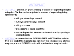
The hand (manus) is a part of the upper limb and includes the wrist, the metacarpus and fingers.
Fingers are usually referred as the thumb, the index, the middle, the ring and the small finger as
represented in fig. 1. Few structures of the human anatomy are so unique as the hand. The hand
needs to present high mobility in order to allow the proper position of the fingers and thumb. Adequate
strength resulting from complex coordination and control methods forms the basis for normal hand
function, as it allows the development of fine motor tasks with high-precision and different gripping
strategies.
2.1.
Skeletal bone structure
Bones are skeletal supporting structures that allow the transmission of the internal loads, provide
stiffness to the skeletal structure and together with the joints contribute for a proper gross motion of
the hand. There are 27 bones within the wrist and hand distributed by 3 major areas: the carpal, the
metacarpal and the phalangeal. The wrist itself contains eight small bones, called carpals, which are
showed in fig. 1: the hamate (1), the pisiform (2), the triquetrum (3), the capitate (4), the lunate (5), the
scaphoid (6), the trapezium (7), and the trapezoid (8). All carpal bones participate in wrist function
5
except the pisiform, which is a sesamoid bone through which the flexor carpi ulnaris tendon passes.
The scaphoid serves as link between each row and therefore, it is vulnerable to fractures. The distal
row of carpal bones is strongly attached to the base of the second and third metacarpals, forming a
fixed unit. All other structures (mobile units) move in relation to this stable unit. The flexor retinaculum,
which attaches to the pisiform and hook of hamate ulnarly, and to the scaphoid and trapezium radially,
forms the roof of the carpal tunnel.
The carpals connect to the metacarpals. There are five metacarpals forming the palm of the hand.
Each metacarpal is characterized as having a base, a shaft, a neck, and a head. One metacarpal
connects to each finger and thumb. The first metacarpal bone (thumb) is the shortest and most
mobile. Each finger (excluding the thumb) includes the distal phalange, the middle phalange and the
proximal phalange. The thumb only has one interphalangeal joint between the two thumb phalanges,
respectively the distal phalange and the proximal phalange.
The three phalanges in each finger (without the thumb) are separated by two joints, called
interphalangeal joints (IP joints), whose major physiological characteristics will be further described in
section 2.4.
Distal
phalange
PHALANGES
Middle
phalange
Distal
phalange
Proximal
phalange
Proximal
phalange
1
8
METACARPAL
7
2
CARPAL
3
4
Fig. 1. Bones of the hand
6
5
6
2.2. Muscles and tendons
The muscles of the hand are divided into intrinsic and extrinsic muscle groups. The intrinsic
muscles are located within the hand itself, whereas the extrinsic muscles are located proximally in the
forearm and insert into the hand skeleton by long tendons.
2.2.1
Extrinsic extensor muscles
The extensor muscles are all extrinsic except for the interosseous-lumbrical complex involved in
interphalangeal joint extension. All the extrinsic extensor muscles are innervated by the radial nerve.
This group of muscles consists of 3 wrist extensors and a larger group of thumb and digit extensors as
represente in fig. 2 and fig. 3.
Fig. 2. Partial view of the muscles of the hand
The extensor carpi radial brevis (ECRB) is the main extensor of the wrist, along with the extensor
carpi radialis longus (ECRL) and extensor carpi ulnaris (ECU), which also deviate the wrist radially
and ulnarly, respectively. The ECRB inserts at the base of the third metacarpal, while the ECRL and
ECU insert at the base of the second and fifth metacarpal, respectively.
The extensor digitorum communis (EDC), extensor indicis proprius (EIP), and extensor digiti minimi
(EDM) extend the digits. They insert to the base of the middle phalanges as central slips and to the
base of the distal phalanges as lateral bands. The abductor pollicis longus (APL), extensor pollicis
brevis (EPB), and extensor pollicis longus (EPL) extend the thumb. They insert at the base of the
thumb metacarpal, proximal phalanx, and distal phalanx, respectively.
7
The extensor retinaculum (ER) prevents bowstringing of tendons at the wrist level and separates
the tendons into 6 compartments. The extensor digitorum communis (EDC) is divided in a series of
tendons to each digit with a common muscle belly and with intertendinous bridges between them. The
index and small finger each have independent extension function through the extensor indicis proprius
(EIP) and extensor digiti minimi (EDM).
Adductor pollicis
Abductor
digiti
minimi
brevis
Opponens
Digiti minimi
Flexor
digiti
minimi
brevis
Flexor pollicis
brevis
Opponens
pollicis
Adductor pollicis
brevis
Interrosei
Fig. 3. Partial view of the muscles of the hand
2.2.2
Extrinsic flexors
The extrinsic flexors consist of 3 wrist flexors and a larger group of thumb and digit flexors. They
are innervated by the median nerve, except for the flexor carpi ulnaris (FCU) and the flexor digitorum
profundus (FDP) to the small and ring finger, which are innervated by the ulnar nerve.
The flexor carpi radialis (FCR) is the main flexor of the wrist, along with the flexor carpi ulnaris
(FCU) and the palmaris longus (PL), which is absent in 15% of the population. They insert at the base
of the third metacarpal, the base of the fifth metacarpal, and the palmar fascia, respectively. The FCU
is primarily an ulnar deviator. The 8 digital flexors are divided in superficial and deep muscle groups.
Along with the flexor pollicis longus (FPL), which inserts at the thumb distal phalanx, they pass
through the carpal tunnel to provide flexion at the interphalangeal joints.
At the palm, the flexor digitorum superficialis (FDS) tendon lies superficial to the palm of the hand.
It then splits at the level of the proximal phalanx and reunites dorsal to the profundus tendon to insert
8
in the middle phalanx. The flexor digitorum profundus (FDP) perforates the superficialis tendon to
insert at the distal phalanx. The relationship of flexor tendons to the wrist joint, metacarpophalangeal
joint and interphalangeal joint is maintained by a retinacular or pulley system that prevents the
bowstringing effect.
2.2.3
Intrinsic muscles
The intrinsic muscles are situated totally within the hand. They are divided into 4 groups: thenar,
hypothenar, lumbrical, and interossei muscles.
The thenar group consists of the abductor pollicis brevis (APB), flexor pollicis brevis (FPB),
opponens pollicis (OP), and adductor pollicis (AP) muscles. All are innervated by the median nerve
except for the adductor pollicis and deep head of the flexor pollicis brevis, which are innervated by the
ulnar nerve. They originate from the flexor retinaculum and carpal bones and insert at the thumb's
proximal phalanx.
The hypothenar group consists of the palmaris brevis (PB), abductor digiti minimi (ADM), flexor
digiti minimi (FDM), and opponens digiti minimi (ODM). They are all innervated by the ulnar nerve.
This group of muscles originates at the flexor retinaculum and carpal bones and inserts at the base of
the proximal phalanx of the small finger.
The lumbrical muscles contribute to the flexion of the metacarpophalangeal joints and to the
extension of the interphalangeal joints. They originate from the flexor digitorum profundus tendons at
the palm and insert on the radial aspect of the extensor tendons at the digits. The index finger
lumbricals (IFL) and long finger lumbricals (LFL) are innervated by the median nerve, and the small
finger lumbricals (SFL) and ring finger lumbricals (RFL) are innervated by the ulnar nerve.
The interossei group consists of 3 volar and 4 dorsal muscles, which are all innervated by the ulnar
nerve. They originate at the metacarpals and form the lateral bands with the lumbricals. The dorsal
interossei (DI) abduct the fingers, whereas the volar interossei (VI) adduct the fingers to the hand axis.
2.3.
Neurological structure
The hand is innervated by 3 nerves, the median, the ulnar, and the radial nerves respectively. Each
has both sensory and motor components. Variations from the classic nerve distribution are so
common that they are the rule rather than the exception. The skin of the forearm is innervated
medially by the medial antebrachial cutaneous nerve and laterally by the lateral antebrachial
cutaneous nerve.
The median nerve is responsible for innervating the muscles involved in the fine precision and
pinch function of the hand. It originates from the lateral and medial cords of the brachial plexus (C5T1) and extends until the fingers. In the forearm, the motor branches supply the pronator teres, flexor
9
carpi radialis, palmaris longus and flexor digitorum superficialis muscles. The anterior interosseus
branch innervates the flexor pollicis longus, flexor digitorum profundus (index and long finger) and
pronator quadratus muscles.
Muscles of thenar
eminences
Fig. 4. The thenar eminences
Proximal to the wrist, the palmar cutaneous branch provides sensation at the thenar eminence
(fig. 4)
As the median nerve passes through the carpal tunnel, the recurrent motor branch innervates the
thenar muscles (abductor pollicis brevis, opponens pollicis, and superficial head of flexor pollicis
brevis). It also innervates the index and long finger lumbrical muscles. Sensory digital branches
provide sensation to the thumb, index, long, and radial side of the ring finger.
The ulnar nerve is responsible for innervating the muscles involved in the power grasping function
of the hand. It originates at the medial cord of the brachial plexus (C8-T1) and extends until the
fingers. Motor branches innervate the flexor carpi ulnaris and flexor digitorum profundus muscles to
the ring and small fingers. Proximal to the wrist, the palmar cutaneous branch provides sensation at
the hypothenar eminence. The dorsal branch, which branches from the main trunk at the distal
forearm, provides sensation to the ulnar portion of the dorsum of the hand and small finger, and part of
the ring finger.
At the hand, the superficial branch forms the digital nerves, which provide sensation at the small
finger and ulnar aspect of the ring finger. The deep motor branch passes through the Guyon canal in
company with the ulnar artery. It innervates the hypothenar muscles (abductor digiti minimi, opponens
10
digiti minimi, flexor digiti minimi, and palmaris brevis), all interossei, the 2 ulnar lumbricals, the
adductor pollicis, and the deep head of the flexor pollicis brevis.
The radial nerve is responsible for innervating the wrist extensors, which control the position of the
hand and stabilizes the fixed unit. It originates from the posterior cord of the brachial plexus (C6-8). At
the elbow, motor branches innervate the brachioradialis and extensor carpi radialis longus muscles. At
the proximal forearm, the radial nerve divides into the superficial and deep branches. The deep
posterior interosseous branch innervates all the muscles in the extensor compartment, namely the
supinator, the extensor the carpi radialis brevis, the extensor digitorum communis, the extensor digiti
minimi, the extensor carpi ulnaris, the extensor indicis proprius, the extensor pollicis longus, the
extensor pollicis brevis and the abductor pollicis longus. The superficial branch provides sensation at
the radial aspect of the dorsum of the hand, the dorsum of the thumb, and the dorsum of the index,
long, and radial half of the ring finger proximal to the distal interphalangeal joints.
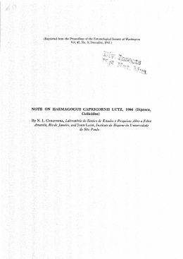
2.4.Joints and ligaments
The hand is composed by 3 types of articular joints: the wrist joint complex with the intercarpal
joints, the metacarpophalangeal joints and the interphalangeal joints as depicted in fig. 5.
The
interphalangeal
joints
The metacarpophalangeal
jonts
The wrist joint
Complex(intercarpal joints)
Fig. 5. Joints of the hand
11
The wrist joint is a complex multiarticulated joint that allows wide range of motion in flexion,
extension, circumduction, radial deviation, and ulnar deviation. The distal radioulnar joint allows
pronation and supination of the hand as the radius rotates around the ulna. The radiocarpal joint
includes the proximal carpal bones and the distal radius. The proximal row of carpals articulates with
the radius and ulna to provide extension, flexion, ulnar deviation, and radial deviation. This joint is
supported by an extrinsic set of strong palmar ligaments that arise from the radius and ulna. Dorsally,
it is supported by the dorsal intercarpal ligament between the scaphoid and triquetrum and by the
dorsal radiocarpal ligament.
At the intercarpal joints, motion between carpal bones is very restricted. These joints are supported
by strong intrinsic ligaments. The most important ones are the scapholunate ligament and the
lunotriquetral ligament. Disruption of either one can result in wrist instability. The Gilula lines have
been described to represent the smooth contour of a greater arc formed by the proximal carpal bones
and a lesser arc formed by the distal carpal bones in normal anatomy. All 4 distal carpal bones
articulate with the metacarpals at the carpometacarpal (CMC) joints. The second and third CMC joints
form a fixed unit while the first CMC forms the most mobile joint.
At the metacarpophalangeal joints, lateral motion is limited by the collateral ligaments, which are
actually lateral oblique in position rather than true lateral. This arrangement allows the ligaments to be
tight when the joint is flexed and loose when extended. The volar plate is part of the joint capsule that
attaches only to the proximal phalanx, allowing hyperextension. The volar plate is the site of insertion
for the intermetacarpal ligaments. These ligaments restrict the separation of the metacarpal heads.
At the interphalangeal joints, extension is limited by the volar plate, which attaches to the
phalanges at each side of the joint. Radial and ulnar motion is restricted by collateral ligaments, which
remain tight through their whole range of motion. Knowledge of these configurations is of great
importance when splinting a hand in order to avoid joint contractures.
12
Chapter 3
Common Pathologies and Injuries of the Human
Hand
In this chapter the most common pathologies of the human hand are described. This brief
description is provided for the sake of understanding the problem of the rehabilitation of the hand and
the driven concepts for the construction of the prototype of the hand rehabilitation.
The upper limbs have a large number of different genetic and environment derived abnormalities,
some of which can be surgically repaired, while others may indicate other syndromes or karyotype
anomalies by association. Many of the hand abnormalities are described as dactyly from the Greek
(daktulos) for finger or digit.
3.1.
The congenital defects of the hand
The congenital defects of the hand happen seldom. For example, acheiria is a missing hand,
adactyly is the absence of the metacarpal (or metatarsal), amelia is a complete absence of a limb and
aphalangia, showed on the fig. 6, is the absent of one or more digit fingers.
Fig. 6. Partial aphalangia of the right upper limb
13
The brachydactyly 7.a) is when middle phalanges of both hands are very short in length or absent.
Ectrodactyly, showed on the fig. 7.b), is a split or cleft hand.
Fig. 7. a) Branchydactyly, b) Ectrodactyly
Trisomy 21 or Down Syndrome (fig. 8) features short and broad hands with clinodactyly (curving of
the fifth finger, little finger), a single flexion crease (20%) and hyperextensible finger joints (UNSW,
2008).
Fig. 8. Trisomy 21- hand features
In the makrodaktylia one finger is bigger than the remaining and in the mikrodaktylia, is the
opposite.
14
Polydactyly also called polydactylia or polydactylism (fig. 9) is when more than 5 fingers can be
found in the hand. This condition is often treated surgically in the infant. Polydactyly can also be
associated with a number of different syndromes including Greig cephalopolysyndactyly syndrome
(GCPS) (UNSW, 2008).
Fig. 9. Polydactyly
Syndactyly (fig. 10) is a fusion of fingers which may be single or multiple and may affect skin only,
skin and soft tissues or skin, soft tissues and bone. The condition is unimportant in toes but disabling
in fingers and requires operative separation and is frequently inherited as an autosomal dominant
(UNSW, 2008).
Fig. 10. Syndactyly
15
3.2. Major hand injures
Hand injuries can be simple or complex. A lot of injures to the hand comes from sports, physical
works and falls. Hand injures are usually not life threatening but without meticulous care, they can be
the source of considerable disability.
3.2.1.
Hand wounds
Because hand wounds are not life threatening, the priority for evacuation and early surgery is low.
For example the injury (fig. 11) may seem serious. But this fingertip injury can easily be attached back
in place by a qualified hand surgeon. The nail bed is protected by an artificial nail splint to allow proper
healing of the nail bed. On the fig. 12 is showed the hand 1 year after the surgery.
Due to the site and depth of injury, the ulnar nerve is injured and results in paralysis of the intrinsic
muscles to the hand. This also resulted in the loss of sensation to the ring and little fingers. Immediate
treatment should be sought to ensure the nerve is repaired. A delayed repair may result in the need
for nerve graft and consequent poorer outcome. In this type of injures rehabilitation is often required.
Fig. 11. Finger injury
Fig. 12. Finger 1 year after the surgery
16
3.2.2.
Tendon Injuries
Other biological structures that often damage in a hand injury are the tendons. Tendons are
collagen cables that help bending and straighten the fingers, since the muscles which move the
fingers are located up in the forearm. It is therefore the tendon that connects the joints of the fingers to
the muscles. The most common and difficult problem that people have after a tendon injury is the loss
of the ability to fully bend or straighten the finger.
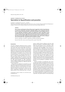
Depending on the timing, surgery can be done to repair or graft the tendon. Acute injuries require
repair and late diagnosis may result in the need for grafting. On figs. 13 to 19 examples are showed of
missed tendon injuries to the right middle and ring finger and the results obtained after the surgery.
Also in this cases, rehabilitation procedures are required in post operative phases (HARMS, 2005).
Fig. 13. Pre-operative absence of extension to the middle and ring fingers
Fig. 14. Operative findings showing loss of the flexor tendons
17
Fig. 15. Harvesting of the palmaris longus tendon graft
Fig. 16. Grafting of the flexor tendons to the middle and ring fingers
Fig. 17. Post operative results after 6 months
Fig. 18. Acute flexor tendon injuries such as this require only a good flexor
tendon repair and hand therapy
18
Fig. 19. Therapy and post-operative results of a 3 finger flexor tendon injuries
3.2.3.
Fractures of the hand
Fractures are also very common injuries to the hand. This type of injuries usually present pain and
swelling. Fractures of the hand may cause permanent deformities. It is usually the intra-articular
fractures (the ones that extend into a joint) that requires immediate or early attention but these
fractures are usually overlooked because they present little deformities and bruising.
Stable fractures can be treated conservatively with closed reduction to restore bone alignment.
Unstable and intra-articular fractures usually require open reduction and internal fixation procedures
for best results (fig. 20) (HARMS, 2005).
Fig. 20. Proximal phalangeal fracture with open reduction and internal fixation done
19
Many hand injuries are the result of a fall. A common injury that occurs in such circumstances wrist
fracture. The wrist is often fractured during a fall on an outstretched arm. In this position, the arm
remains straight and the wrist takes the full force of the fall. While the two bones in the forearm, the
radius and the ulna, are the most likely to fracture, it is also possible that the small bone in the wrist
just behind the base of the thumb, the scaphoid bone, can fracture (fig. 21).
Fig. 21. Ice-skating fall
3.2.4.
Ligament Injuries
Ligament are other biological structures that sustain injuries during a fall. For example during winter
sports injury to the thumb ligament has become one of the more common skiing injuries over the past
20 years. It ranks second only to knee sprains. Skier's thumb is a strain or tear to the thumb's major
stabilizing ligament-the ulnar collateral ligament of the metacarpophalangeal joint of the thumb (fig.
22). The ulnar collateral ligament assists us in grasping, pinching, and stabilizing items in our hands.
Injury to the thumb while skiing usually results from a fall on an outstretched hand that continues to
hold the ski pole. At impact, the thumb is driven directly into the snow and is bent back or to the side,
away from the palm and index finger, straining or tearing the ligament. When injured, the ulnar
collateral ligament and other ligaments cannot support the thumb bone, making grasping or pinching
with the thumb difficult (HHA, 2000).
20
Fig. 22. Skier's thumb
Thumb injuries require evaluation to establish the correct diagnosis and initiate proper treatment.
Physical signs include pain, swelling, and tenderness on the inner side of the metacarpophalangeal
joint and loss of strength in the thumb. X-rays should be taken to rule out damage to the bone.
Sometimes, a small piece of the bone is torn off with the ligament. Treatment for a torn ligament
usually consists of a brief period of wearing a splint or cast for immobilization. Occasionally, however,
with complete tears or displacement of the ligament, surgery is required to repair the injured ligament.
Long-term problems can result from instability of the thumb. With proper treatment, however, the
patient can regain full function and return to activity (HHA, 2000).
3.3.
Diseases of the hand
The hand can be affected by many diseases including muscular and neurological. Many require
rehabilitation. Following is a brief description of the most common ones.
3.3.1.
Hirayama Disease
Hirayama Disease is a juvenile muscular atrophy of the distal upper extremity is a sporadic
juvenile-onset disease that presents with the gradual onset of unilateral weakness and atrophy in the
hand and forearm muscles. Generally, this disorder is considered a benign, non-progressive motor
neuron disease. Operative reconstruction by tendon transfer improved the activities of daily living
(ADL) of a patient with advanced Hirayama disease who showed marked intrinsic muscle atrophy of
the left hand (fig. 23) (Chiba, S., et. al., 2004).
21
Fig. 23. Amyotrophy of left hand
3.3.2.
Dupuytren Disease
Dupuytren's disease most often affects the pretendinous bands or fascia of the hand (see the
normal hand structure on the left). As the disease progresses, these areas can thicken and form a
rope like cord. Eventually, the disease can severely affect the hand's appearance and function,
causing contracture (fig. 24) (RH, 2008)
Fig. 24. Dupuytren’s disease
22
3.3.3.
Partial paresis
Partial paresis of the hand causes the atrophy of muscles (see fig. 25)
Fig. 25. Partial paresis of the finger
3.3.4.
Arthritis
Arthritis (fig. 26) is a generic term for inflammatory joint disease. Regardless of the cause,
inflammation of the joints may cause pain, stiffness, swelling, and some redness of the skin about the
joint.
Fig. 26. An elderly woman's hand deformed by severe arthritis
23
3.3.5.
Carpal Tunnel Syndrome
Carpal tunnel syndrome (fig. 27) is a narrow bony passage in the wrist formed by the bones of the
wrist (carpal bones) on the bottom and the transverse carpal ligament on the top. An important nerve
(median nerve) and nine tendons that allow the wrist to flex, or move downward, pass through this
small area. Carpal tunnel syndrome (CTS) occurs when the median nerve, the softest structure in the
tunnel, becomes compressed against the transverse carpal ligament. The median nerve is responsible
both for the ability to fire the nine tendons to flex the wrist and for sensation in certain fingers in the
hand.
Fig. 27. Carpal tunnel syndrome
24
Chapter 4
Multibody Systems with Natural Coordinates
In the scope of this work, a multibody system is an assembly two or more planar rigid bodies (also
called elements) that can be joined together, in such a way that their relative movement became
constrained. The joining of two rigid bodies is called a kinematic pair or simply a joint (Nikravesh, P.,
1988), (Haug, E., 1989). A joint permits certain degrees of freedom or relative motion and prevents or
restricts others. Joint are classified in classes. In planar multibody systems there are 2 classes of
Joints: a class I joint allows one degree of freedom, (e.g. a revolute or hinge joint (R) allows one
relative rotation), a class II joint allows two degrees of freedom (e.g. a revolute-translational joint (R-T)
allows one relative rotation and one relative translation).
Multibody systems are classified as open-chain of closed-chain systems. If a system is composed
of bodies without closed branches (or loops), then it is called an open-chain system, otherwise, it is
called a closed-chain multibody system.
Multibody System can be also acted up on by external forces. Forces can be conservative like the
gravitational acceleration field or non-conservative like the friction force.
4.1.
Dependent and Independent Coordinates
In order to describe a multibody system, the first important point to consider is that of choosing a
mathematical way of describing its position and motion. In other words, select a set of coordinates that
will allow one to unequivocally define the position, velocity, and acceleration of the multibody system
at all times.
There can be two choices in terms of coordinate selection: independent coordinates (fig. 28),
whose number coincides with the number of degrees of freedom of the multibody system and is
thereby minimal, or dependent coordinates (fig. 29) in a number larger than that of the degrees of
freedom of the system and with which can the multibody system be much more easily described,
25
although interrelated through certain algebraic equations known as constraint equations. In most
cases independent coordinates are not a suitable solution for a general purpose analysis, because
they do not meet one important requirement: the coordinate system should unequivocally define the
position of the multibody system. In fact independent coordinates directly determine the position of the
input bodies of the value of the externally driven coordinates, but not the position of the entire system.
Therefore additional non-trivial analysis need be performed to this end.
Fig. 28. Independent coordinates – system of 2 particles: The system of particles (1 and 2)
has 4 degrees of freedom (x1, y1, x2, y2). The displacements x1, y1, x2, y2 are
independent coordinates in the system of the 2 particles.
Alternatively, dependent coordinates (fig. 29) generate a number of constraints that is equal to the
difference between the number of dependent coordinates and the number of degrees of freedom.
Constraint equations are generally nonlinear, and play a mjor role in the kinematics and dynamics of
multibody systems. These type of coordinates are the alternative choice to the independent set of
coordinates as they uniquely determine the position of all bodies. Three major types of coordinates
have been proposed to solve this problem: relative coordinates, reference point or Cartesian
coordinates, and natural or fully Cartesian coordinates. In this work, natural or fully Cartesian
Coordinates is the solution adopted to describe the multibody system under analysis.
In the case of planar multibody systems, natural coordinates can be considered as an evolution of
the reference point coordinates in which the points are moved to the joints or to other important points
of the elements, so that each element has at least two points. It is important to point out that since
each body has at least two points, its position and angular orientation are determined by the Cartesian
coordinates of these points, and the angular variables used by reference point coordinates are no
longer necessary.
Thus the natural coordinates in the case of planar multibody systems are made of Cartesian
coordinates of a series of points.
26
y
1(x 1 ,y1 )
2(x 2 ,y2 )
x
Fig. 29. Rigid body with 2 points - dependent coordinates: the system uses 4 coordinates.
However a planar body has only 3 degrees of freedom. x1, y1, x2, y2 are related
as the length need to be kept.
4.2.
Kinematics Analysis
Kinematics problems are of a purely geometrical nature and can be solved, regardless of the forces
and inertia characteristics of elements. Kinematic analysis aims to calculate the position and
orientation of all elements of the system, during the analysis period, giving the position of its elements.
Input elements of a multibody system as those whose position or motion is know or specified.
The position and motion of the other elements of the system are found in accordance with the position
and motion of the input elements. There are as many input elements as there are degrees of freedom
for the multibody system.
Kinematic Analysis provides a view of the entire range of motion of a multibody system. The
solution of the kinematics simulation encompasses the calculation of the position, velocity and
acceleration of the system. It also permits one to detect collisions, study the trajectories of points,
analyze the position of an element of the multibody system and calculate the rotation angles of the
driving elements.
4.2.1.
Initial position and finite displacement analysis
The initial position or assembly problem consist in finding the position of all the elements of the
multibody system once that of the input elements is known. This problem difficult to solve, since it
leads to a system of nonlinear algebraic equations which has, in general, several possible solutions.
Finite displacement problem is a variation of the initial position problem. Given a fixed position on
the multibody system and a known finite displacement (not infinitesimal) for the input bodies (or
elements), the problem of finite displacements consists of finding the final position of the system’s
27
remaining bodies. This problem will be easier to solve than initial position, mainly because one starts
from a known position of the system, which can be used as a starting point for the iterative process
needed for the solution of the resulting nonlinear equations.
As seen before, dependent coordinates generate a set of algebraic constraint equation that
represent the interdependency between these coordinates.
Defining the vector of generalized
coordinates q as the vector that holds all the dependent coordinates, then, the solution of the
Kinematic problem resides in obtaining the solution of:
Φ(q,t)=0
(4.1)
where Φ is the global Kinematic constraint vector , i.e., the vector that contains all the Kinematic
Constraint equations of the system, in the homogeneous form. As there are several constraints that
are used to define the inputs of the system in time
Φ (q,t)=0 can explicitly depend on t.
It is customary to resort to the well-know Newton-Raphson method, which has quadratic
convergence in the neighborhood of the solution and does not usually cause serious difficulties if one
starts with a good initial approximation, to solve eq. (4.1). The Newton-Raphson method is based on a
linearization of eq. (4.1) and consists in replacing this system of equations with the first two terms of its
expansion in a Taylor series around a certain approximation qi of the desired solution:
Φ(qi,t)+ Φq(q-qi)=0
(4.2)
where matrix Φ q is the Jacobian matrix of the constraint equations, that is to say, the matrix of partial
derivatives of these equations with respect to the dependent coordinates. Eq. (4.2) must be solved
iteratively until a solution is found or in other words, when
qi+1-qi =∆qi≤ ε ≅ 0
(4.3)
where previous equation represents the iterative procedure of the Newton-Raphson method, and ε is a
user specified error tolerance.
4.2.2.
Velocity and Acceleration analysis
Velocity and Acceleration Analysis is much easier to solve than the position problems, mainly
because it is linear and has a unique solution. This means in mathematical terms that it is modelled by
a system of linear equations.
Calculation of the velocities and accelerations of the system considers that if there can not exist
violation of the associated kinematic constraint equations (4.1), then, the same must also holds true
for the velocities and accelerations associated to these constraints, i.e:
28
& (q, q& , t ) = 0
Φ
(4.4)
&& (q, q& , q
&&, t ) = 0
Φ
(4.5)
for the velocities , and
for the accelerations.
Expanding eq. (4.4) and (4.5) the following equations are obtained:
Vector
ν = −Φ t = −
Φ q (q)q& = −Φ t ≡ ν
(4.6)
& −Φ
& q& ≡ γ
&& = −Φ
Φ q (q)q
t
q
(4.7)
∂Φ
is referred to as the rigid-hand-side of the velocity constraint equations.
∂t
& q& is referred to as the vector of the rigid-hand-side of the acceleration constraint
Vector γ = ν& − Φ
q
equation where
&& is the vector of generalized
q& is the vector of generalized dependent velocities, and q
dependent accelerations.
4.3.
Dynamic Analysis
Dynamic analyses are much more complicated to solve than kinematic ones. The major
characteristic about dynamic problems is that they involve the forces that act on the multibody system
and its inertial characteristics namely its mass, inertia tensor and the position of its centre of gravity.
There are essentially two types of dynamic analysis: Inverse Dynamic Analysis and Forward Dynamic
Analysis: The inverse dynamic problem aims at determining the motor of driving forces that produce a
specific motion, as well as the reactions that appear at each one of the multibody system’s joints. It is
necessary to know the velocities and accelerations to be able to estimate the inertia forces which,
together with the weight, the forces in the spring and dampers and all the other known external forces,
will provide the basis to calculate the required actuating forces. The forward dynamic problem
(Dynamic Simulation) yield the motion of a multibody system over a given time interval, as a
consequence of the applied forces and given initial conditions. The importance of the direct dynamic
problem lies in the fact that it allows one to simulate and predict the system’s actual behaviour; as the
motion is always the result of the forces that produce it.
29
4.3.1.
Equations of Motion of a Multibody System
There are several ways of obtaining the equations of motion of a multibody system. In this work
one first considers the system of two unconstrained rigid bodies described in figure 30 a).
i
j
i
j
Fig. 30. a) Unconstrained system of rigid bodies, b) constrained system of rigid bodies
According to Newton-Euler equations, the equations of motion of such a system can be written as:
&& = g
Mq
(4.8)
where g is generalized external force vector and M is the mass matrix containing the mass and inertial
characteristics of each rigid body.
If a set of constraint bodies is considered instead, as depicted in figure 30b) them the equation of
motion will become:
&& + g (i) = g
Mq
(4.9)
where an additional term g(i) is added representing the generalized internal force vector arising from
the kinematic constraints imposed to the system. Using the Lagrange multiplier’s method, these forces
can be expressed as a function of the Jacobian matrix (that provides the direction of these forces) and
a vector
λ of unknown Lagrange multipliers (that describes their magnitude) as:
g (i) = Φ qT λ
(4.10)
Substituting eq. (4.10) in eq. (4.9), the resulting equation of motion becomes
&& + Φ qT λ = g
Mq
&& are unknown, it is necessary to add equation (4.12) to solve this problem:
Because λ and q
30
(4.11)
&& = γ
Φqq
(4.12)
resulting the final expression of the system of the equations of motion of the model:
&& + Φ qT λ = g
⎧⎪Mq
⎨
&& = γ
⎪⎩ Φ q q
(4.13)
In matrix form, equation (4.13) becomes:
⎡M
⎢
⎢⎣Φ q
&&⎫ ⎧q ⎫
Φ qT ⎤ ⎧⎪q
⎥⎨ ⎬ = ⎨ ⎬
0 ⎥⎦ ⎪⎩λ ⎭ ⎩γ ⎭
(4.14)
The equation of motion of the system (4.14) must be integrated in time in order to obtain the
response of the model. This is done considering an Initial Value Problem (IVP) and the method
proposed by (Nikravesh, P., 1988).
4.3.2.
Mass Matrix
The form of mass matrices will undoubtedly depend on the type of coordinates chosen for the
representation of multibody system. In this work, the use of Natural Coordinates lead to an elaborated
deduction of this matrix that remains outside the scope of this work. The interested reader is referred
to the work of (Jalón, J. and Bayo, E., 1994).
The mass matrix of a general planar rigid body, described with 2 points, is given by:
2mxG
⎡
⎢m − L
ij
⎢
⎢
0
⎢
M=⎢
⎢ mxG − I i
⎢ Lij
L2ij
⎢
⎢ − my G
⎢⎣
Lij
0
2mxG
Lij
my G
Lij
mxG I i
− 2
Lij
Lij
m−
mx G I i
− 2
Lij
Lij
my G
Lij
Ii
L2ij
0
my G ⎤
Lij ⎥
⎥
mxG I i ⎥
− 2⎥
Lij
Lij
⎥
⎥
0
⎥
⎥
Ii
⎥
⎥⎦
L2ij
−
(4.15)
where Ii is polar moment of inertia with respect to the basic point i, m is mass of the element (rigid
body), Lij is lengths of the body, xG , y G are the coordinates of the centres of masses with respect to
the point i.
31
4.3.3.
External forces
The application of external concentrated forces in a multibody formulation with Natural
Coordinates requires a transformation of Coordinates that describes the concentrated force F, applied
at point P (with coordinates rp) by an equivalent generalized force ge distributed by the points defining
the rigid body, given by:
g e = CTF
(4.16)
where ge is the generalized force of the element , F is the external concerted force and C the
transformation matrix given by:
⎡( 1 − c1 ) c 2 c1 − c 2 ⎤
C=⎢
⎥
⎣− c 2 ( 1 − c1 ) c 2 c1 ⎦
(4.17)
With c1, c2 numerical coefficient calculate from the local coordinates of point P in the rigid body’s
reference frame. The interested reader is referred to the work of (Jalón, J. and Bayo, E., 1994) for a
more comprehensive description of the calculation of matrix C.
32
Chapter 5
Multibody Model of the Hand and
Rehabilitation Device
As it was seen in Chapter 3, there are many pathologies that can affect the human hand:
congenital defects, several types of hand injures (including factures), tendon and ligament injures and
hand diseases. All of these pathologies interfere directly with the hand function and movement as they
produce damage in the neurological and musculo-skeletal structure of the hand. Hand rehabilitation
can be accomplished using proper rehabilitation devices. These devices are able to improve hand
function and movement, restoring (in many cases) its normal activity. There are already several
different types of hand rehabilitation devices as it can be seen next in this chapter. Each device serves
a specific purpose on hand rehabilitation.
In this chapter a computational model of a new rehabilitation device is constructed using the
multibody formulation described in Chapter 4 with natural coordinates. This type of computational
models are important in all phases of the design of a new product, but its application is particularly
relevant in the early design phase when no prototype is yet available.
5.1.
Hand rehabilitation devices
Although a search for hand rehabilitation devices reveals that there are already available in the
market several different types of models, with different function and purposes, it is also true that there
is still a lot to develop in this field.
Hand may suffer from many pathologies, as seen briefly in a previous chapter, therefore several
solutions are available. For example, to the rehabilitation of the palm discs are being used (fig. 31a) or
balls (fig. 31b). The ball (fig. 32a) or the mesh (fig. 32b) are used for the rehabilitation of the fingers.
To the rehabilitation of the wrist the powerball (fig. 33) is one possible solution.
33
Fig. 31. a) Discs, b) The ball
Fig. 32. a) The ball, b) Meshes
Fig. 33. Powerball
34
5.2
Scope of Application of the Hand Rehabilitation Device Under
Development
The rehabilitation device that is now proposed is specially aimed to help patients with partial
paresis of the fingers acquired after a Cerebral Vascular Accident (CVA), although more general
applications can be considered.
The device under development is presented in figure 34. There one can see the physical prototype
made of wood and rope and its virtual counterpart made in the geometrical modeler Unigraphix 5.0.
Fig. 34. a) Physical prototype, b) Virtual prototype
The device is conceived for active practices of the hand allowing the resistance relief of the rectifier
muscles of the fingers. The resistive force is generated by a set of weights that are hanged in strings
that attach to each finger. This weight may vary from person to person and from pathology to
pathology. The attachment of the strings to the fingers is made using a simple velcro stripe. The
device allows both hands to work although it can be used independently for each hand. Hands are
firmly immobilized using proper hand immobilizer. The position of the vertical support can be tuned to
meet patient’s anthropometrics.
5.3.
The Multibody Model
Considering the biomechanical system to analyse, represented in fig. 34a) and composed by the
hand, lower arm and rehabilitation device, the decision (in terms of constructing a planar multibody
model will natural coordinates capable of describing the physical one), is to consider that the lower
arm is irrelevant for the analysis and that it can be removed if the kinematics of the wrist were properly
considered. Therefore the model includes the hand, starting at the metacarpus and finishing in the
distal phalange of the indicate finger, as depicted on fig. 34a) and 34b). The interaction with the
rehabilitation device is only considered in dynamic terms and is considered by introducing a constant
35
force with magnitude equal to the gravitational force produced by the weight and variable direction
prescribed by the unit vector going from the attachment point of the hand to the attachment point in
the device.
P6 = P7
R3
IV
P8
D2 = y 8 (t )
III
P4 = P5
D4 = θ 3 (t )
D3 = θ 4 (t )
D5 = θ 2 ( t )
8
2
=
3
D1 = x8 (t )
R2
D6 = θ1 (t )
II
P2 = P3
R1
I
P1
Fig. 35. Multibody model of the hand: 4 rigid bodies (I to IV), eight points (P1 to P8). Three
revolute joints (R1-R3) and 6 degree-of-freedom (D1 to D6)
5.3.1.
Natural coordinates, kinematic constraints and degrees-of-freedom
As it can be observed from fig. 35, the multibody model is described by four rigid bodies (the
metacarpal, the proximal phalange, the middle phalange, the distal phalange) interconnected by 3
revolute joints. Considering that each rigid body requires 2 points to be properly described and that
revolute joints are explicitly described by 2 independent points, then the model requires a total number
of 8 points, (i. e., 16 natural coordinates) that are put together in vector:
{
q = x1 , y1 , x 2 , y 2 , x3 , y 3 , x 4 , y 4 , x5 , y 5 , x6 , y 6 , x7 , y 7 , x8 , y8 }(16 x1)
T
(5.1)
A closer analysis of the proposed model reveals that it possesses 6 degrees-of-freedom,
respectively the 2 translations and 1 rotation of the wrist joint and the 3 rotations of the revolute joints.
Therefore, the number of required kinematic constraints, required to express the dependencies among
the Natural Coordinates is equal to the difference between the number of coordinates and the number
of the system’s degrees of freedom, i. e., 16-6=10 kinematic constraints.
36
These kinematics constraints (including the ones that drive the system) are presented hereafter
and expressed by algebraic equations with different natures: 4 kinematics constraint equations of rigid
body type that are used to preserve the constant length of rigid bodies I to IV; 6 kinematic constraint
equations of revolute joint type that are used to describe the 3 revolute joints; and 6 kinematic
constraint equations of kinematic drivers type that are used to fully prescribe the motion of the system
during the kinematics and dynamics analyses preformed.
In analytical terms, these equations are represented as:
ƒ
Rigid body type (constant length):
Body I:
2
Φ 1 = r12T ⋅ r12 − L12
= ( x 2 − x1 ) 2 + ( y 2 − y1 ) 2 = 0
(5.2)
Body II:
Φ 2 = r34T ⋅ r34 − L234 = ( x 4 − x3 ) 2 + ( y 4 − y 3 ) 2 = 0
(5.3)
Body III:
Φ 3 = r56T ⋅ r56 − L256 = ( x6 − x5 ) 2 + ( y 6 − y 5 ) 2 = 0
(5.4)
Body IV:
Φ 4 = r78T ⋅ r78 − L278 = ( x8 − x7 ) 2 + ( y8 − y 7 ) 2 = 0
(5.5)
Where the inner product of vector was used to prescribe these relations between the coordinates.
ƒ Revolute joint type:
Joint R1:
⎧ x − x 2 ⎫ ⎧0⎫
Φ 5,6 = r3 − r2 = ⎨ 3
⎬ =⎨ ⎬
⎩ y 3 − y 2 ⎭ ⎩0⎭
(5.6)
Joint R2:
⎧ x − x 4 ⎫ ⎧0⎫
Φ 7 ,8 = r5 − r4 = ⎨ 5
⎬ =⎨ ⎬
⎩ y 5 − y 4 ⎭ ⎩0⎭
(5.7)
Joint R3:
⎧ x − x6 ⎫ ⎧0⎫
Φ 9,10 = r7 − r6 = ⎨ 7
⎬ =⎨ ⎬
⎩ y 7 − y 6 ⎭ ⎩0⎭
(5.8)
ƒ Kinematic drivers type:
Drivers D1 and D2 (translation of point 8):
⎧⎪ x − x8* (t ) ⎫ ⎧0⎫
Φ11,12 = ⎨ 8
⎬ =⎨ ⎬
*
⎪⎩ y8 − y8 (t )⎭ ⎩0⎭
37
(5.9)
Driver D3 (angle of the wrist (fig. 36), called
θ 4 ):
Φ 13 = r78 × X − L78 sin θ 4 (t ) = −( y 7 − y 8 ) − L78 sin θ 4 (t ) = 0
(5.10)
,
( x7 , y7 )
θ 4 (t )
X = (1,0 )
( x8 , y8 )
Fig. 36. The hand with the angle in the wrist
Driver D4 (angle between the metacarpal and the proximal phalange (fig.37) called
θ 3 ):
Φ 14 = r78 × r65 − L78 ⋅ L65 ⋅ sin θ 3 =
= −( y8 − y 7 ) ⋅ ( x5 − x6 ) + ( x8 − x7 ) ⋅ ( y 5 − y 6 ) − L78 ⋅ L56 ⋅ sin θ 3 (t ) = 0
(5.11)
( x6 , y6 )
,
x7(, xy7 )
P6 (=
6
( x8* (t ), y8* (t ))
θ 3 (t )
D4 =
3
( x5 , y 5 )
(x8 , y8 )
Fig. 37. The hand with the angle
θ3
Driver D5 (angle between proximal phalange and middle phalange (fig. 38) called
θ 2 ):
Φ 15 = r56 × r43 − L56 ⋅ L43 ⋅ sin θ 2 (t ) =
= −( y 6 − y 5 ) ⋅ ( x3 − x 4 ) + ( x6 − x5 ) ⋅ ( y 3 − y 4 ) − L56 ⋅ L43 ⋅ sin θ 2 (t ) = 0
38
(5.12)
,
P6 (=x6(, xy66 )
( x5 , y5 )
( x8* (t ), y8* (t ))
D4 =
( x4 , y4 )
3
θ 2 (t )
(x3 , y3 )
Fig. 38. The hand with the angle
θ2
Driver D6 (angle between the middle phalange and the distal phalange (fig. 39) called
θ1 ):
Φ 16 = r34 × r21 − L34 ⋅ L21 ⋅ sin θ1 (t ) =
= −( y 4 − y 3 ) ⋅ ( x1 − x 2 ) + ( x 4 − x3 ) ⋅ ( y1 − y 2 ) − L34 ⋅ L12 ⋅ sin θ1 = 0 (5.13)
,
P4 = (x4 , y4 )
P3 = (x3 , y3 )
P2 = (x2 , y2 )
D6 = θ1(t)
P1 = (x1, y1)
Fig. 39. The hand with the angle
39
θ1
The kinematic constraints presented before are grouped together in vector
Φ , the vector of global
kinematic constraint expressed as:
2
⎧( x 2 − x1 ) 2 + ( y 2 − y1 ) 2 − L12
⎫
⎪
⎪
2
2
2
⎪( x 4 − x3 ) + ( y 4 − y 3 ) − L34
⎪
⎪( x − x ) 2 + ( y − y ) 2 − L2
⎪
5
6
5
56
⎪ 6
⎪
⎪( x8 − x7 ) 2 + ( y8 − y 7 ) 2 − L278
⎪
⎪
⎪
⎪ x3 − x 2
⎪
⎪y − y
⎪
2
⎪ 3
⎪
⎪ x5 − x 4
⎪
⎪⎪
⎪⎪
y − y4
Φ(q, t ) = ⎨ 5
⎬=0
−
x
x
⎪ 7
⎪
6
⎪y − y
⎪
6
⎪ 7
⎪
⎪ x8 − x8 * (t )
⎪
⎪
⎪
⎪ y8 − y8 * (t )
⎪
⎪− ( y 7 − y8 ) ⋅ 1 + ( x7 − x8 ) ⋅ 0 − L78 ⋅ sin(θ 4 * (t ))
⎪
⎪
⎪
⎪− ( y 4 − y 3 )( x1 − x 2 ) + ( x 4 − x3 )( y1 − y 2 ) − L43 ⋅ L21 ⋅ sin(θ1 * (t )) ⎪
⎪− ( y − y )( x − x ) + ( x − x )( y − y ) − L ⋅ L ⋅ sin(θ * (t ))⎪
6
5
3
4
6
5
3
4
65
43
2
⎪
⎪
⎪⎩− ( y8 − y 7 )( x5 − x6 ) + ( x8 − x7 )( y 5 − y 6 ) − L78 ⋅ L56 ⋅ sin(θ 3 * (t )) ⎪⎭
A closer analysis of vector
(5.14)
Φ(q,t ) reveals that all constraints are either quadratic or linear in the
coordinates, which represents an advantages from the computation point of view inherent to this type
of formulation.
5.3.2.
Jacobian matrix
As it was seen before, the Jacobian matrix (table 1) plays one of the most important roles in
kinematic and dynamic analyse of a multibody system. By definition the Jacobian matrix is the partial
derivative of the vector of global kinematic constraints in order to the generalise coordinates vector. In
the case of Natural Coordinates, and considering that the kinematic constraints are either quadratic or
linear, their contribution to this matrix will be linear or constant in the coordinates, respectively. For the
case of the multibody model of the hand, the Jacobian matrix assumes the following form:
40
Table 1 Jacobian Matrix
41
5.4.
Contributions to the ν and γ vectors
General expressions for vector
υ
and
γ
were provided in Chapter 4. These vector present the right-
hand side of the velocity and acceleration constraint equations respectively.
The only non-zero entries of the vector ν are the ones associated with the drivers constraints as
these are the only ones explicitly depending on time. Therefore the contributions of the kinematic
constraints for the computational multibody model of the hand are respectively:
⎧
0
⎫
⎪
⎪
0
⎪
⎪
⎪
⎪
0
⎪
⎪
0
⎪
⎪
⎪
⎪
0
⎪
⎪
0
⎪
⎪
⎪
⎪
0
⎪
⎪
0
⎪
⎪
ν=⎨
⎬
0
⎪
⎪
⎪
⎪
0
⎪
⎪
x& 8* (t )
⎪
⎪
⎪
⎪
y& 8* (t )
⎪
⎪
⎪ L78 cos(θ 4 (t )) ⋅ θ&4 (t ) ⎪
⎪ L ⋅ L cos(θ (t )) ⋅ θ& (t ) ⎪
3
3
⎪ 78 65
⎪
&
⎪ L65 ⋅ L43 cos(θ 2 (t )) ⋅ θ 2 (t )⎪
⎪
& ⎪
⎩ L43 ⋅ L21 cos(θ 1 (t )) ⋅ θ 1 (t ) ⎭
(5.15)
The calculation of the contributions for vector γ are more elaborated as they represent a 2nd derivative,
although also because of this motive, the contributions of linear constraints are null. For the
computational
model
of
the
hand,
the
respectively:
42
contributions
for
γ
vector
are
⎫
⎧− 2[( x& 2 − x&1 ) + ( y& 2 − y& 1 )]
⎪
⎪− 2[( x& − x& ) + ( y& − y& )]
4
3
4
3
⎪
⎪
⎪
⎪− 2[( x& 6 − x& 5 ) + ( y& 6 − y& 5 )]
⎪
⎪
⎪
⎪− 2[( x& 8 − x& 7 ) + ( y& 8 − y& 7 )]
⎪
⎪0
⎪
⎪
⎪
⎪0
⎪
⎪0
⎪
⎪
⎪
⎪0
⎪
⎪
γ = ⎨0
⎬
⎪
⎪
⎪0
⎪
⎪ &x&* (t )
⎪ (5.16)
⎪ 8
⎪
⎪ &y&8* (t )
⎪
⎪
⎪
2
⎪ L78 ⋅ (− sin(θ 4 (t ))) ⋅ θ&4 (t ) + cos θ 4 (t ) ⋅ θ&&4 (t )
⎪
⎪
⎪
2
&
&&
⎪ L78 ⋅ L65 ⋅ (− sin θ 3 (t )) ⋅ θ 3 (t ) + cos θ 3 (t ) ⋅ θ 3 (t ) − 2 ⋅ (−( y& 8 − y& 7 ) ⋅ ( x& 5 − x& 6 ) + ( x& 8 − x& 7 ) ⋅ ( y& 5 − y& 6 ) ⎪
⎪ L ⋅ L ⋅ (− sin θ (t )) ⋅ θ& 2 (t ) + cos θ (t ) ⋅ θ&& (t ) − 2 ⋅ (−( y& − y& ) ⋅ ( x& − x& ) + ( x& − x& ) ⋅ ( y& − y& )⎪
2
2
2
2
6
5
3
4
6
5
3
4
⎪ 65 43
⎪
2
⎪⎩ L43 ⋅ L21 ⋅ (− sin θ 1 (t )) ⋅ θ&1 (t ) + cos θ 1 (t ) ⋅ θ&&1 (t ) − 2 ⋅ (−( y& 4 − y& 3 ) ⋅ ( x& 2 − x&1 ) + ( x& 4 − x& 3 ) ⋅ ( y& 2 − y& 1 ) ⎪⎭
5.5.
Kinematic Data Collection
In order to analyze the movement of the hand a set of 4 flexion – extension hand movements were
collected using the BTS (Body Training Systems) system with six cameras in the Laboratory of
Biomechanics of the Silesian University of Technology in Poland.
The movement acquisition consisted in recording the coordinates of a set of 7 markers (6 in the
lower arm and hand and 1 in the rehabilitation device) as depicted in fig. 40. The subject was a
healthy young female with 23 years old and with no hand pathologies. The measured lengths of the
subject’s hand were very similar with the ones found when averaging the reconstructed values
obtained from the BTS system and therefore these average lengths were use instead of the measured
ones with the purpose of comparing the kinematics obtained with the driven multibody model with the
kinematics obtained directly from the movement laboratory. In table 2 the average lengths are
provided, together with the mass and inertial characteristics which are introduced in the next
subsection.
43
Fig. 40. Markers on the hand
The markers were recorded with a sampling frequency of 120Hz and the 3D coordinates of the
points reconstructed automatically by the software package of the BTS system. The four flexionextension movements of the hand had a duration of 11.2 sec.
System’s drivers, respectively the coordinates of the wrist point and the interphalangeal angles
( θ 1 to
θ 4 ), were calculated from this kinematic data using an excel worksheet.
The results obtained, especially for the angles were very noisy and therefore a filtering procedure
was required. In this work a Butterworth 2nd order filter was used to filter the kinematic drivers (Winter,
D., 1990). The filter applies the double-pass technique to avoid the phase lag introduced by this type
of filters. Residual Analysis was applied for an estimation of the cut off frequencies (Winter, D., 1990)
but the results suggested by this method failed to produce good results due to the still high levels of
noise in the kinematic data. Therefore, cut-off frequencies of 1.5 – 2.3Hz were obtained by trial and
error methods and successfully applied in the filtering of the kinematic data.
5.6.
Masses, Inertias and assembly of the Global Mass Matrix
The dynamic analysis of the hand requires the prescription of the hand masses and inertias to the
dynamic multibody program.
The hand is a very complex system of bones, soft tissues and joints and therefore it is not easy to
obtain, or even estimate, those values.
A search in the available literature also confirm the scarcity of such data, although the values for
the masses could be obtained form (Biryukova, V. and Yourovskaya, 1994).These values are
44
presented in Table 2 together with the values of the length, radius and polar inertias of the 4 rigid
bodies of the model. It was consider that the total mass of the hand was 1 kg.
Table 2. Parameters included in model
Body
Mass [kg]
Length [m]
Radius [m]
Inertias [kg m2 ]
I
0.007
0.02101
0.0075
1.128x10-6
II
0.014
0.01910
0.0075
1.899x10-6
III
0.030
0.03008
0.010
9.798x10-6
IV
0.662
0.07717
0.015
1.351x10
-3
The masses presented in previous table include the masses of the corresponding bones plus the
masses of all adjoining muscles (Biryukova, V., and Yourovskaya, 1994). The polar inertias were
calculated using the approximation to a solid cylinder given the expression
I = ml 2 / 3 + mr 2 / 4 . The
center of mass of each rigid body was considered to be located in the middle of each rigid segment.
The global mass matrix of the multibody system results of the assembly of the four elementar mass
matrices, provided in Chapter 4, for each one of the rigid bodies. Since there are no sharing of points,
because the revolute joints are explicitly define, the global mass matrix is band diagonal and
uncoupled:
45
Table 3. Mass matrix
46
5.7.
Kinetic Data
Kinetic data refers to the values of external forces and moments applied upon the system. In this
case, since the movement occurs in a plane perpendicular to the direction of the earth gravitational
field, the gravitational force is not applied.
Therefore according to fig. 41 the only external force acting on the system is the one applied by
the string and corresponding weight. The magnitude of this force is always constant and equal to
F=mw g and its direction is coincident with the direction followed by the string. The origin of the string
(attached to the finger) is moving and its insertion (at the device) is fixed. The force is applied to the
model following the procedure described in Chapter 4.
Fig. 41. Force generate by the finger
5.8. Results of the Kinematic and Dynamic Analysis of the Multibody Model
of the Hand
The model described before was implemented in two Matlab programs, following the formulation
presented in Chapter 4.
The first Matlab program (HAND_Kinematics.m) deals only with the Kinematic aspect of the
moment under analysis and is able to calculate the position, velocity and acceleration of the system in
47
any instant of the analysis. This program was implemented in the initial part of this work and its source
code can be found in Annex 4. Since it is only a Kinematic program, it does not use masses, inertias
and external forces.
For a complete dynamic analysis a second Matlab program was implement (HAND_Dynamic.m)
that besides the calculation of the positions, velocities and accelerations of the system, it also allows
the calculation of the reaction forces at the joints and the articular moments of force that muscles need
to develop around each joint in order for the prescribed motion to occur. The source code of this
program can be found in Annex 5. In fig. 42a the initial position of the hand with respect to the
rehabilitation device is presented. This figure was obtained from the Matlab program and respects the
initial animation frame. Also a film sequence is presented in fig. 42b regarding one flexion-extension
cycle.
a)
b)
Fig. 42. a) Initial position of the hand, b) Kinematic sequence of animation of the flexion-extension movement
48
5.8.1.
Analysis Indicators
& and
One way to verify if the analysis is working properly is to calculate the norm of vectors Φ, Φ
&& at each time step. If constraints are being respected and if the Baumgarte stabilization is working,
Φ
properly, then these values should be close to zero.
From the results presented in fig. 43, it is clear that from the kinematics point of view, the
conditions imposed by the constraint equations are being respected as the values of the norms of
& and Φ
&& are always smaller than 1.5x10-7, 8.0x10-6 and 1.0x10-4 respectively. Values in abscissa
Φ, Φ
represent frame numbers.
Fig. 43. Analysis statistics
5.8.2.
Drivers of the Multibody Model
In figure 44 the values that were calculated from the kinematic data for the drivers of the system
are presented. The filtered values of the driver are interpolated using cubic splines and their
respective velocities and accelerations calculated by cubic spline differentiation.
49
Fig. 44. Kinematic drivers for the analysis: angles, angular velocity and angular acceleration of each joint
The results clearly show the four flexion-extension cycles of the hand. It also can be seen that
drivers far away from the wrist joint present a more noisy behavior, indicating that lower-cut-off
frequencies could have been used.
The results in terms of drivers, velocities and accelerations also show that these quantities are
consistent with drivers positions and velocities respectively.
The Kinematics analysis of the drivers also show that maximum flexion-extension angular velocities
oscillate between 0.5 rad/s for the wrist joint to 4 rad/s for the metacarpal-phalangeal joint. Values of
1 rad/s to 2 rad/s can be found for the maximum angular velocities of the top and middle
interphalangeal joints, respectively.
50
5.8.3.
Kinematic Analysis
In this section the results of the kinematic analysis of the hand biomechanical model are presented.
In figures 45-52 the positions, velocities and accelerations of each of the 8 points of the model are
presented.
From the analysis of the results it can be seen that in terms of positions, these are consistent with
the kinematic data obtained from the laboratory indicating that the drivers are working properly.
Moreover, it can also be observed that the velocities are compatible with positions, and accelerations
with velocities.
The values for the velocities and accelerations are within the expected physiological range for a
normal hand. In absolute values velocities never exceed 0.2 m/s for any of the points independently of
the hand being flexing or extending.
Accelerations are still a bit noisy especially for points further away from the wrist, indicating that
probably smaller cut-off frequencies could have been used. However, in absolute values,
accelerations never surpass 2.0 m/s2 and in many cases they are bellow 0.5 m/s2. These results are
within the expected range accelerations for a hand with no pathologies.
The comparison of the kinematics of the two points of a revolute joint reveals that they are equal,
meaning that the joint kinematic constraints are working properly.
Fig. 45. Kinematics for point 1
51
Fig. 46. Kinematics for point 2
Fig. 47. Kinematics for point 3
52
Fig. 48. Kinematics for point 4
Fig. 49. Kinematics for point 5
53
Fig. 50. Kinematics for point 6
Fig. 51. Kinematics for point 7
54
Fig. 52. Kinematic for point 8
5.8.4.
Dynamic Analysis
In this section the dynamic related results are presented. These refer to the reaction forces at the
joints (presented in fig. 53) and the articular moments of force at the joints (fig. 54).
A closer observation of the first results show that reactions in revolute joint R1 are practically null.
That was to be expected since no gravity is considered in this planar movement and that there is no
external forces applied to body I. The small variations observer in the reaction force represent the
inertial components due to the dynamics of the body.
In the revolute joints R2 and R3 (and also at the wrist attachment point) one can see that the
reaction forces are following the direction and the magnitude of the external applied force. This results
was expected since there are no gravitational component present and inertia forces are small since
accelerations are also small, and proves that the model is working probably in terms of the calculation
of the joint reaction forces.
55
Fig. 53. Reactions of the hand
In figure 54 the articular moments generated at the joints during the movement are presented. This
is probably the most relevant result of this study as it allows the analysis of the performance of the
hand rehabilitation device.
The first obvious observation is that the moments at the joint R1 is almost zero, since no forces are
applied to body I.
Then, observing the other graphics, it is clear that moments have similar behavior in all joints but
with a tendency to grow as one approximates the wrist joint. That is understandable since as we are
moving away from the point of application of the force the arm of the moment increases.
Another result that can be observed and that is important for the analysis of the efficiency of the
rehabilitation device is that all moment of force are positive (higher values correspond to maximum
extension, lower values to maximum flexion). This means that even when flexing, the hand is trying to
sustain the weight load and therefore an eccentric contraction of the hand extensors is occurring
instead of a contraction of the hand flexors. If any flexor activity is present it is in co-contraction with
the hand extensor, with the purpose of stabilizing the movement.
56
Previous sentence moreover can only be corroborated if a muscular analysis is preformed, in order
to calculate the redundant muscle forces, which, although important, remains outside the scope of this
work. Regarding the calculation of the redundant muscles forces the interested reader is referred to
the work of (Silva, et. al., 2002a, Silva, et. al., 2002b).
Fig. 54. Moments in each joint
57
Chapter 6
Conclusion and Future Developments
6.1.
Conclusions
In this work a computational model for the kinematic and dynamic analysis of 2D hand motions was
presented using a multibody formulation with natural coordinates. In the framework of the proposed
methodology, two problems have been analyzed: kinematic problems to study the movement of the
hand, and dynamic problems to study internal forces and articular moments. The procedures
presented use reliable and accurate mathematical methodologies, that have the remarkable
advantage of being able to obtain, without using intrusive techniques, qualitative and quantitative
results regarding the human hand structure and motion.
A comprehensive mathematical model of the human hand was assembled and thoroughly
described, using a general-purpose multibody formulation in which the position and orientation of the
human hand is represented using natural or fully Cartesian coordinates.
This formulation, was chosen among other types of coordinates due to the advantages it presents
in the description of biomechanical systems. It was observed that since rigid segments of the human
hand are modelled as a collection of points, it becomes very convenient, in biomechanical
applications, to use the location of important anatomical landmarks, such as joints and extremities,
directly in the construction of the rigid bodies describing the anatomical segments of the
biomechanical model.
Two model-specific gross-motion analysis programs were developed in the MATLAB environment,
using the described multibody formulation with fully Cartesian coordinates. These numerical tools
were the computational support for all the kinematic and dynamic analyses performed in this work.
59
It was seen that the model was able to correctly characterize the principal physical characteristics
and anthropometric dimensions of the human hand. The investigation was done on a healthy hand to
which a weight was attached to the middle phalange to produce an external force during the motion
executed in the prototype device. Although, during the investigation the wrist was supposed to be
fixed, the acquired movement revealed a displacement of the wrist of about 2cm. This displacement
was properly included in the model using a moving attachment point in the wrist joint.
The kinematics were obtained in the movement laboratory and properly filtered using a 2nd Order
Butterworth low-pass filter to remove excessive noise levels.
The input kinematics for the kinematic model proved to be consistent with the experimental data
and correct physiological values were obtained for the angles and angular velocities at the joints.
It was seen that the reactions at the joints have a constant magnitude (equal to the force produced
the weight attached to the finger) but changing direction, fact that directly interferes with the produced
moment at the articulations as the moment arm changes accordingly.
Regarding the articular moments, it was conclude that during the 4 flexion-extension cycles, these
moments were always positive, meaning that, with the actual design, only hand extensors are
rehabilitated.
As a final conclusion, it can be stated that the model developed in this work was able to analyse
the actual design of the rehabilitation device and can be easily adapted to analyse other design
alternatives.
6.2.
Future Developments
The model proposed is robust but simple. This means that there are other important features that
can be implement in the future.
For the analysis of the rehabilitation of the hand it would be important to analyse the activation
patterns and forces produced by the muscles to rehabilitate. This feature was not included in the
present work as it would require the implementation of optimization tools with which the redundant
force sharing problem could be solved.
Also it would be important to include more fingers in the model and extend it to 3D to take full
advantages of the data collected by the BTS System.
With such a model, it would also be important to compare the results it produces with muscular
Electromyography (EMG) patterns measured in the principal muscle groups.
60
References
Biryukova, V. and Yourovskaya, Z., “A model of human hands dynamics”, from Schuind F, Coorney III
W.P., Garcia-Elias M: “Advances in the Biomechanics of the Hand and Wrist”, New York, NATO
ASI Series, 1994.
Chen, F., Lo, S., Meng, N., Lin, C., Chou, L.,: “Effects of wrist position and contraction on wrist flexors
H-reflex, and its functional implications.”, Journal of Electromyography and Kinesiology, 16, 2006.
Chiba,S., Yonekura,K., Nonaka, M., Imai, M., Matumoto, H., and Wada, T., "Advanced Hirayama
Disease with Successful Improvement of Activities of Daily Living by Operative Reconstruction"
vol. 25,no1, 2004.
Coburn, J., Upal, M., Crisco, J., “Coordinate systems for the carpal bones of the wrist”, Journal of
Biomechanics, 40, 2007.
Ettema, A., An, K., Zhao, C., O’Byrne, M., Amadio, P., “Flexor tendor and synovial gliding during
tunnel syndrome”, Journal of Biomechanics, 41, 2008.
Feltham, M., Dieen, J., Coppieters, M., Hodges, P., “Changes in joint stability with muscle contraction
measured from transmission of mechanical vibration”, Journal of Biomechanics, 39, 2006.
Gielo-Perczak, K., “Biomechanical analysis of the wrist joint in ergonomical aspect”, from Schuind F,
Coorney III W.P, Garcia-Elias M: “Advances in the Biomechanics of the Hand and Wrist”, New
York, NATO ASI Series, 1994.
Halaki, M., O’Dwyer, N., Cathers, I.,: “Systematic nonlinear relations between displacement amplitude
and joint mechanics at the human wrist”, Journal of Biomechanics, 39, 2006.
Haug, E.,: Computer Aided Kinematics and Dynamics of Mechanical Systems, Allyn and Bacon,
Boston, 1989.
Jalón, J. and Bayo, E., Kinematic and dynamic simulation of multibody systems : the real-time
challenge, Springer-Verlag, New York ; Hong Kong, 1994.
Kuo, P., Lee, l., Jindrich, D., Dennerlein, J., “Finger joint coordination during tapping”, Journal of
Biomechanics, 39, 2006.
61
Nelson, D., Margaret, A., Mitchell, P., Groszewski, G., Pennick, S., Manske, P., “Wrist range of motion
in activities of daily living”, from Schuind F, Coorney III W.P, Garcia-Elias M: “Advances in the
Biomechanics of the Hand and Wrist”, New York, NATO ASI Series, 1994.
Nikravesh, P., Computer-aided analysis of mechanical systems, Prentice-Hall, Englewood Cliffs, N.J.,
1988.
Seeley R., Stephens T., Tate P., Anatomy & Physiology. McGraw Hill, 2006.
Silva, M. and Ambrósio, J., "Kinematic Data Consistency in the Inverse Dynamic Analysis of
Biomechanical Systems", Multibody System Dynamics, 8(2), 219-239, 2002a.
Silva, M. and Ambrósio, J., "Solutions of Redundant Muscle Forces in Human Locomotion with
Multibody Dynamics and Optimization Tools", Journal of Mechanics Based Design of Structures
and Machines, 31(3), 381-411, 2002b.
Tortora, G., Grabowski, S. R., Introduction to the Human Body, J. Wiley, NY, 2001.
Valero-Cuevas, J:, “An integrative approach to the biomechanical function and neuromuscular control
of the fingers”, Journal of Biomechanics, 38, 2005
Vigouroux, L., Quaine, F., Labarre-Vila, A., Moutet, F:, “Estimation of finger muscle tendon tensions
and pulley forces during specific sport-climbing grip techniques”, Journal of Biomechanics, 39,
2006.
Winter, D.,: Biomechanics and motor control of human movement, Wiley, New York, 1990.
Wu, G., Helm, F., Veeger, D., Makhsous, M., Roy, P., Anglin, C., Nagels, J., Karduna, A., McQuade,
K., Werner, W., Buchholz, B.,: “ISB recommendation on definitions of joints coordinate systems of
various joints for the reporting of human joint motion – Part II: shoulder, elbow, wrist and hand”,
Journal of Biomechanics, 38, 2005.
Relevant Internet References :
ACPOC, http://www.acpoc.org/library/1976_05_017.asp, June 2008
CHARMS, http://www.charmssingapore.com/hand_injuries.php, 2005
DofOS, http://www.naika.or.jp/im2/43/01/16c.aspx, September, 2003
HHA, http://www.hughston.com/hha/a_14_1_2.htm, 2000
UNSW Embryology, http://embryology.med.unsw.edu.au/Notes/skmus72.htm, 2008
62
Annex 1
Sizes and masses of hand links
63
Fig. 55. Model of the hand
Table 4. Sizes and masses of links in the model (Biryukova, V. and Yourovskaya, Z., 1994)
Link No
1
2
3
4
5
6
7
8
9
10
11
12
13
14
15
16
Link length [m]
0.451
0.260
0.237
0.254
0.243
0.196
0.173
0.150
0.150
0.121
0.173
0.121
0.168
0.121
0.121
0.116
65
Masses [kg]
0.662
0.121
0.030
0.033
0.022
0.018
0.022
1.014
0.014
0.007
0.016
0.007
0.015
0.007
0.007
0.004
Annex 2
Maximum values of wrist joint capacity
67
Table 5. Maximum values of wrist joint capacity with the AUR profiles 1-4 during
performance of activities I-X. (Chen, F., Lo, S., Meng, N., Lin, C., Chou, L., 2007)
Value for each activity [Nm]
No. of
I
II
III
IV
V
VI
VI
VIII
IX
X
1
66
78
122
84
0
155
0
18
354
22
2
50
88
0
63
0
102
0
16
192
20
3
67
112
124
85
0
156
0
18
0
23
4
74
309
134
93
105
169
0
61
187
26
profiles
Fig. 56. The typical of activities performed at the assembly line in lamp factory study
69
Annex 3
Wrist range of motion activities of daily living
71
Table 6. Wrist Range of Motion in Activities of Daily Living (Nelson, D., Margaret, A.,
Mitchell, P., 1994)
Radial [deg]
Ulnar[deg]
Flexion [deg]
Extension [deg]
Activity
Max
Min
Avg
max
min
avg
max
min
avg
max
min
avg
Comb hair
18
-3
10.4
44
8
29.9
74
14
38.4
55
32
42.2
Tailbone
24
-3
11.6
37
12
24.3
65
28
49.8
66
-5
37.8
Washcloth
15
-6
6.4
50
17
34.4
74
9
28.3
65
25
49.2
Button
14
-5
6.3
40
7
19.1
35
-5
20.3
47
10
29.4
Tie shoe
15
2
7.5
31
13
22.7
56
-2
17.9
45
17
29.3
Use knife
17
-18
-7.1
37
16
26.4
32
-25
2.9
37
-5
15.0
Use fork
16
-9
-0.1
37
12
23.7
22
-20
-4.8
55
28
38.6
Spatula
2
-25
-12.1
45
25
37.2
44
8
25.4
53
12
28.9
Drink cup
11
-10
0.5
45
18
32.8
6
-27
-11.0
44
19
31.8
Pitcher
12
-3
6.1
42
17
31.2
36
-15
5.3
61
29
46.6
Can opener
18
-15
4.2
33
16
25.3
10
-22
-5.7
53
22
41.3
Stir bowl
18
-30
5.4
43
10
33.8
56
15
32.5
56
-8
21.6
Open jar
25
-10
6.9
47
32
39.6
57
24
35.3
52
12
34.8
Turn faucet
18
-2
9.0
51
27
40.0
50
18
26.3
59
-4
29.6
Turn page
17
-19
0
45
6
27.5
52
-17
17.7
40
8
28.3
Write name
13
-18
0.9
38
-8
11.6
10
-50
-20.0
54
14
33.9
Use phone
17
-3
9.2
32
15
24.7
10
-19
-3.2
63
37
51.1
Dial “O”
17
-23
0
28
11
24.6
30
-5
10.8
54
7
28.8
Typewriter
17
7
11.4
46
18
29.3
42
0
22.0
50
10
36.2
Steer wheel
11
-2
4.7
45
28
34.9
35
-9
9.2
65
17
39.3
Door knob
11
-25
-8.3
44
26
36.3
20
-18
-1.1
54
24
41.2
Turn key
5
-22
-9.4
47
19
34.6
10
-36
-1.7
45
14
33.5
Screwdriver
-12
-25
-18.0
45
18
34.8
25
-9
2.5
45
23
33.4
Throw ball
18
-5
6.2
37
13
24.6
31
6
16.4
64
30
48.1
73
Annex 4
Hand Kinematics – Matlab Program Source
75
HAND_kinematics.m
%
%
%
%
Begin
Program to analyze the kinematic of the hand
This is 2D
Date:
% Variable declaration
clear all;
clc;
close all;
nc
= 16;
nh
= 10;
nd
= 6;
nh_total = nh+nd;
q
= zeros(nc,1);
q_dot
= zeros(nc,1);
q_2dot = zeros(nc,1);
Phi = zeros(nh_total,1);
Phi_q = zeros(nh_total,nc);
niu=zeros(nh_total,1);
gamma=zeros(nh_total,1);
% Model's data
L1=0.025;%m
L2=0.017;%m
L3=0.035;%m;
L4=0.085;%m;
L=[L1 L2 L3 L4];
errorUser=1*10^-5;
%Analysis data:
t0 = 0.0
dt = 1/10;
t_end = 11.4;
load drivers.txt;
n=size(drivers,1);
%Begin Kinematic Analysis
t = t0;
q=[0.369055-0.0199980.348411-0.0183530.348411-0.0183530.329179-0.0159080.3291790.0159080.300538-0.0173630.300538-0.0173630.222256-0.008233]';
while t<=t_end
% Position analysis with Newton-Raphson method
error=errorUser;
while error>=errorUser
[Phi,Phi_q,
niu,gamma]=Function_evaluation(t,q,q_dot,Phi,Phi_q,L,drivers,niu,gamma,nc,nh_total,
nd);
delta_q=-Phi_q\Phi;
error=sqrt(delta_q' *delta_q);
q=q+delta_q;
end
% Velocity analysis
q_dot=Phi_q\niu;
77
% Acceleration analysis
q_2dot=Phi_q\gamma;
% Animate results
newplot;
hold on;
axis ([0.0 0.5 -0.25 0.25]); axis equal; axis manual;
for j=1:nc/2
x(j,1) = q(1+2*(j-1),1);
y(j,1) = q(2+2*(j-1),1);
end
plot(x,y);
clear x,y;
pause(0.1);
hold off;
% Increment time variable
t=t+dt
end
78
Function_Evaluation.m
function
[Phi,
Phi_q,
niu,
gamma,
drv_t]=Function_evaluation(t,q,q_dot,Phi,Phi_q,L,drivers,niu,gamma,nc,nh_total,nd)
% Getting data
q15_pp
dq15dt_pp
ddq15dt2_pp
from drivers - building the piecewise polinomials
= spline (drivers(:,2),drivers(:,3));
= mmspder(q15_pp);
= mmspder(dq15dt_pp);
q16_pp
dq16dt_pp
ddq16dt2_pp
= spline (drivers(:,2),drivers(:,4));
= mmspder(q16_pp);
= mmspder(dq16dt_pp);
theta1_pp
= spline (drivers(:,2),drivers(:,5));
dtheta1dt_pp
= mmspder(theta1_pp);
ddtheta1dt2_pp = mmspder(dtheta1dt_pp);
theta2_pp
= spline (drivers(:,2),drivers(:,6));
dtheta2dt_pp
= mmspder(theta2_pp);
ddtheta2dt2_pp = mmspder(dtheta2dt_pp);
theta3_pp
= spline (drivers(:,2),drivers(:,7));
dtheta3dt_pp
= mmspder(theta3_pp);
ddtheta3dt2_pp = mmspder(dtheta3dt_pp);
theta4_pp
= spline (drivers(:,2),drivers(:,8));
dtheta4dt_pp
= mmspder(theta4_pp);
ddtheta4dt2_pp = mmspder(dtheta4dt_pp);
% Evaluation of the spline for time t
q15_data
= ppval(t,q15_pp);
q16_data
= ppval(t,q16_pp);
theta1_data
= ppval(t,theta1_pp);
theta2_data
= ppval(t,theta2_pp);
theta3_data
= ppval(t,theta3_pp);
theta4_data
= ppval(t,theta4_pp);
drv_t(1,1)
= q15_data;
drv_t(2,1)
= q16_data;
drv_t(3,1)
= theta1_data;
drv_t(4,1)
= theta2_data;
drv_t(5,1)
= theta3_data;
drv_t(6,1)
= theta4_data;
% Drivers velocities for time t
dq15dt_data
= ppval(t,dq15dt_pp);
dq16dt_data
= ppval(t,dq16dt_pp);
dtheta1dt_data
= ppval(t,dtheta1dt_pp);
dtheta2dt_data
= ppval(t,dtheta2dt_pp);
dtheta3dt_data
= ppval(t,dtheta3dt_pp);
dtheta4dt_data
= ppval(t,dtheta4dt_pp);
drv_t(7,1)
= dq15dt_data;
drv_t(8,1)
= dq16dt_data;
drv_t(9,1)
= dtheta1dt_data;
drv_t(10,1)
= dtheta2dt_data;
drv_t(11,1)
= dtheta3dt_data;
drv_t(12,1)
= dtheta4dt_data;
% Drivers accelerations for time t
ddq15dt2_data
= ppval(t,ddq15dt2_pp);
ddq16dt2_data
= ppval(t,ddq16dt2_pp);
79
ddtheta1dt2_data
ddtheta2dt2_data
ddtheta3dt2_data
ddtheta4dt2_data
drv_t(13,1)
drv_t(14,1)
drv_t(15,1)
drv_t(16,1)
drv_t(17,1)
drv_t(18,1)
=
=
=
=
=
=
=
=
=
=
ppval(t,ddtheta1dt2_pp);
ppval(t,ddtheta2dt2_pp);
ppval(t,ddtheta3dt2_pp);
ppval(t,ddtheta4dt2_pp);
ddq15dt2_data;
ddq16dt2_data;
ddtheta1dt2_data;
ddtheta2dt2_data;
ddtheta3dt2_data;
ddtheta4dt2_data;
% Kinematic constraints evaluation
Phi(1) = (q(3)-q(1))^2+(q(4)-q(2))^2-L(1)^2;
Phi(2) = (q(7)-q(5))^2+(q(8)-q(6))^2-L(2)^2;
Phi(3) = (q(11)-q(9))^2+(q(12)-q(10))^2-L(3)^2;
Phi(4) = (q(15)-q(13))^2+(q(16)-q(14))^2-L(4)^2;
Phi(5) = (q(5)-q(3));
Phi(6) = (q(6)-q(4));
Phi(7) = (q(9)-q(7));
Phi(8) = (q(10)-q(8));
Phi(9) = (q(13)-q(11));
Phi(10) = (q(14)-q(12));
Phi(11) = (q(15)-q15_data);
Phi(12) = (q(16)-q16_data);
Phi(13) = (q(14)-q(16))-L(4)*sin(theta4_data);
Phi(14)
=
-(q(16)-q(14))*(q(9)-q(11))+(q(15)-q(13))*(q(10)-q(12))L(4)*L(3)*sin(theta3_data);
Phi(15)
=
-(q(12)-q(10))*(q(5)-q(7))+(q(11)-q(9))*(q(6)-q(8))L(3)*L(2)*sin(theta2_data);
Phi(16)
=
-(q(8)-q(6))*(q(1)-q(3))+(q(7)-q(5))*(q(2)-q(4))L(2)*L(1)*sin(theta1_data);
% Jacobian matrix evaluation:
Phi_q=zeros(nh_total,nc);
Phi_q(1,1)
= -2*(q(3)-q(1));
Phi_q(1,2)
= -2*(q(4)-q(2));
Phi_q(1,3)
= 2*(q(3)-q(1));
Phi_q(1,4)
= 2*(q(4)-q(2));
Phi_q(2,5)
= -2*(q(7)-q(5));
Phi_q(2,6)
= -2*(q(8)-q(6));
Phi_q(2,7)
= 2*(q(7)-q(5));
Phi_q(2,8)
= 2*(q(8)-q(6));
Phi_q(3,9)
= -2*(q(11)-q(9));
Phi_q(3,10) = -2*(q(12)-q(10));
Phi_q(3,11) = 2*(q(11)-q(9));
Phi_q(3,12) = 2*(q(12)-q(10));
Phi_q(4,13) = -2*(q(15)-q(13));
Phi_q(4,14) = -2*(q(16)-q(14));
Phi_q(4,15) = 2*(q(15)-q(13));
Phi_q(4,16) = 2*(q(16)-q(14));
Phi_q(5,3)
= -1;
Phi_q(5,5)
= 1;
Phi_q(6,4)
= -1;
Phi_q(6,6)
= 1;
Phi_q(7,7)
= -1;
Phi_q(7,9)
= 1;
80
Phi_q(8,8)
Phi_q(8,10)
Phi_q(9,11)
Phi_q(9,13)
Phi_q(10,12)
Phi_q(10,14)
Phi_q(11,15)
Phi_q(12,16)
Phi_q(13,14)
Phi_q(13,16)
Phi_q(14,9)
Phi_q(14,10)
Phi_q(14,11)
Phi_q(14,12)
Phi_q(14,13)
Phi_q(14,14)
Phi_q(14,15)
Phi_q(14,16)
Phi_q(15,5)
Phi_q(15,6)
Phi_q(15,7)
Phi_q(15,8)
Phi_q(15,9)
Phi_q(15,10)
Phi_q(15,11)
Phi_q(15,12)
Phi_q(16,1)
Phi_q(16,2)
Phi_q(16,3)
Phi_q(16,4)
Phi_q(16,5)
Phi_q(16,6)
Phi_q(16,7)
Phi_q(16,8)
=
=
=
=
=
=
=
=
=
=
=
=
=
=
=
=
=
=
=
=
=
=
=
=
=
=
=
=
=
=
=
=
=
=
-1;
1;
-1;
1;
-1;
1;
1;
1;
1;
-1;
-(q(16)-q(14));
(q(15)-q(13));
(q(16)-q(14));
-(q(15)-q(13));
-(q(10)-q(12));
(q(9)-q(11));
(q(10)-q(12));
-(q(9)-q(11));
-(q(12)-q(10));
(q(11)-q(9));
(q(12)-q(10));
-(q(11)-q(9));
-(q(6)-q(8));
(q(5)-q(7));
(q(6)-q(8));
-(q(5)-q(7));
-(q(8)-q(6));
(q(7)-q(5));
(q(8)-q(6));
-(q(7)-q(5));
-(q(2)-q(4));
(q(1)-q(3));
(q(2)-q(4));
-(q(1)-q(3));
% Evaluation of vector niu:
niu(1) = 0;
niu(2) = 0;
niu(3) = 0;
niu(4) = 0;
niu(5) = 0;
niu(6) = 0;
niu(7) = 0;
niu(8) = 0;
niu(9) = 0;
niu(10) = 0;
niu(11)
niu(12)
niu(13)
niu(14)
niu(15)
niu(16)
=
=
=
=
=
=
dq15dt_data;
dq16dt_data;
L(4)*cos(theta4_data)*dtheta4dt_data;
L(4)*L(3)*cos(theta3_data)*dtheta3dt_data;
L(3)*L(2)*cos(theta2_data)*dtheta2dt_data;
L(2)*L(1)*cos(theta1_data)*dtheta1dt_data;
% Evaluation of vector gamma:
gamma(1) = -2*((q_dot(3)-q_dot(1))^2+(q_dot(4)-q_dot(2))^2);
gamma(2) = -2*((q_dot(7)-q_dot(5))^2+(q_dot(8)-q_dot(6))^2);
81
gamma(3) = -2*((q_dot(11)-q_dot(9))^2+(q_dot(12)-q_dot(10))^2);
gamma(4) = -2*((q_dot(15)-q_dot(13))^2+(q_dot(16)-q_dot(14))^2);
gamma(5) = 0;
gamma(6) = 0;
gamma(7) = 0;
gamma(8) = 0;
gamma(9) = 0;
gamma(10) = 0;
gamma(11) = ddq15dt2_data;
gamma(12) = ddq16dt2_data;
gamma(13)
=
L(4)*(sin(theta4_data)*dtheta4dt_data^2+cos(theta4_data)*ddtheta4dt2_data);
gamma(14)
=
L(4)*L(3)*(sin(theta3_data)*dtheta3dt_data^2+cos(theta3_data)*ddtheta3dt2_data)-2*((q_dot(16)-q_dot(14))*(q_dot(9)-q_dot(11))+(q_dot(15)-q_dot(13))*(q_dot(10)q_dot(12)));
gamma(15)
=
L(3)*L(2)*(sin(theta2_data)*dtheta2dt_data^2+cos(theta2_data)*ddtheta2dt2_data)-2*((q_dot(12)-q_dot(10))*(q_dot(5)-q_dot(7))+(q_dot(11)-q_dot(9))*(q_dot(6)q_dot(8)));
gamma(16)
=
L(2)*L(1)*(sin(theta1_data)*dtheta1dt_data^2+cos(theta1_data)*ddtheta1dt2_data)-2*(-(q_dot(8)q_dot(6))*(q_dot(1)-q_dot(3))+(q_dot(7)-q_dot(5))*(q_dot(2)-q_dot(4)));
82
Annex 5
Hand dynamics – Matlab Program Source
83
HAND_Dynamics.m
%
%
%
%
%
Begin
Program to analize the dynamics of the hand
This is 2D
Date: April-June 2008
IST
% Clears workspace
clear all;
close all;
%
% Model's description
%
nc
= 16;
%
nh
= 10;
%
nd
= 6;
%
nh_total = nh+nd;
%
Number of natural coordinates
Number of holonomic kinematic constraints
Number of degrees of freedom
Total number of constraint equations (including drivers)
% Lengths - average values form the kinematics
L1
= 0.02101;%m
L2
= 0.01910;%m
L3
= 0.03008;%m;
L4
= 0.07717;%m;
L_data = [L1 L2 L3 L4];
% Bone Radius
r1 = 0.0075; %m
r2 = 0.0075; %m
r3 = 0.010; %m
r4 = 0.015; %m
% Mass
M1
M2
M3
M4
M_data
of each body
= 0.007;
= 0.014;
= 0.030;
= 0.662;
= [M1 M2 M3 M4];
%Moment of
J1_G
=
J2_G
=
J3_G
=
J4_G
=
J_G_data =
inertia (cylinder approach: J=(m*l^2)/3+(m*r^2/4))
(M1*L1^2)/3+(M1*r1^2)/4;
(M2*L2^2)/3+(M2*r1^2)/4;
(M3*L3^2)/3+(M3*r1^2)/4;
(M4*L4^2)/3+(M4*r1^2)/4;
[J1_G J2_G J3_G J4_G];
% Local coordinates of the centre of mass of each body
rG(1:2,1) = [L1/2 0.0]';
rG(1:2,2) = [L2/2 0.0]';
rG(1:2,3) = [L3/2 0.0]';
rG(1:2,4) = [L4/2 0.0]';
% External force data
r_mass = [0.2*9.81 2]';
r_force = [0.1*L2
0]';
force on body 2
% weight of 0.2 kg applied over body 2
% local coordinates of point of application of the
%Fixed points coordinates - for animation purposes only
85
r_link
= [0.1 -0.005]';
% coordinates of a point located in the lower arm
r_anchor = [0.114 -0.124]'; % coordinates of the anchor point on the device
%Analysis data:
t0
= 0.0;
dt
= 1/30;
t_end = 11.192;
Baum_data = [ 50.0
50.0 ];
% These are the values of alpha and beta of the
Baumegarte's stabilization procedure
load drivers.txt;
n=size(drivers,1);
%Begin Dynamic Analysis - Defines IVP initial step
q
= [0.369055-0.0199980.348411-0.0183530.348411-0.0183530.329179-0.015908
0.329179-0.0159080.300538-0.0173630.300538-0.0173630.222256-0.008233]';
q_dot = [0.0 0.0 0.0 0.0 0.0 0.0 0.0 0.0 0.0 0.0 0.0 0.0 0.0 0.0
0.0 0.0]';
Y_0
= [q; q_dot];
% Solves the IVP using a Direct Intergration Procedure
t_stat = cputime;
[t , Y] = ode45(@Solve_EofM_ODE45, [t0 t_end], Y_0, [], L_data, M_data, J_G_data,
rG, Baum_data, drivers, r_mass, r_force,r_anchor, nc, nh_total, nd);
% Get values from variables
i_rep
= 1;
w_rep
= 26;
t_report = t0;
for i = 1:size(t)
if t(i) >= t_report
[q_2dot_aux,
lambda_aux,
data_aux]
=
Solve_EofM(t(i),
Y(i,1:nc)',
Y(i,nc+1:2*nc)', L_data, M_data, J_G_data, rG, Baum_data, drivers,
r_mass,
r_force,r_anchor, nc, nh_total, nd);
t_rep(i_rep)
= t(i);
q_rep(i_rep,1:nc)
= Y(i,1:nc);
q_dot_rep(i_rep,1:nc)
= Y(i,nc+1:2*nc);
q_2dot_rep(i_rep,1:nc)
= q_2dot_aux';
% Extracts reaction and internal forces
lambda_rep(i_rep,1:nh_total-6) = lambda_aux(1:nh_total-6,1)';
lambda_rep(i_rep,nh_total-5)
= -lambda_aux(nh_total-5,1);
lambda_rep(i_rep,nh_total-4)
= -lambda_aux(nh_total-4,1);
% Calculates articular moments
lambda_rep(i_rep,nh_total-3)
=
3,1)*L_data(4)*cos(data_aux(10,1));
lambda_rep(i_rep,nh_total-2)
=
2,1)*L_data(4)*L_data(3)*cos(data_aux(9,1));
lambda_rep(i_rep,nh_total-1)
=
1,1)*L_data(3)*L_data(2)*cos(data_aux(8,1));
lambda_rep(i_rep,nh_total)
=
0,1)*L_data(2)*L_data(1)*cos(data_aux(7,1));
data_rep(i_rep,1:w_rep)
= data_aux';
i_rep
= i_rep + 1;
t_report
= t_report + dt;
end
86
-lambda_aux(nh_total-lambda_aux(nh_total-lambda_aux(nh_total-lambda_aux(nh_total-
end
% Get the values for the LAB kinematics
load LabKinematics.txt;
for i = 1:i_rep-1
j=1;
while LabKinematics(j,2)<=t_rep(i)
j=j+1;
end
for k = 1:nc
if LabKinematics(j,2) == t_rep(i)
q_kin(i,k) = LabKinematics(j-1,2+k);
else
q_kin(i,k)
=
LabKinematics(j-1,2+k)
+
(LabKinematics(j,2+k)LabKinematics(j-1,2+k))*(t_rep(i)-LabKinematics(j-1,2))/(LabKinematics(j,2)LabKinematics(j-1,2));
end
end
end
t_stat = (cputime - t_stat)/60;
disp('Analysis done!');
disp('See STATISTICS bellow:');
Iterations = size(t,1)
Elapsed_CPU_time = t_stat
disp('Press ENTER to begin animation of results');
pause
% Animate results
fig = figure;
set(fig,'DoubleBuffer','on');
set(gca,'xlim',[-80 80],'ylim',[-80 80],'NextPlot','replace','Visible','off');
mov = avifile('DynamicAnalysisArticular moments.avi');
for i = 111: 180;
1:size(t_rep')
newplot;
hold on;
title([t_rep(i),i]);
axis ([0.1 0.45 -0.20 0.05]); axis equal; axis manual;
% Plot the LAB Kinematics
for j=1:nc/2
x(j,1) = q_kin(i,1+2*(j-1));
y(j,1) = q_kin(i,2+2*(j-1));
end
plot(x,y,'-o','Color',[0.5 0.5 0.5],'LineWidth',1,'MarkerEdgeColor',[0.5 0.5
0.5],'MarkerFaceColor','w');
clear x y;
%
% Plot
x(1,1) =
y(1,1) =
x(2,1) =
y(2,1) =
x(3,1) =
y(3,1) =
the string and force vector
r_anchor(1,1);
r_anchor(2,1);
data_rep(i,25);
data_rep(i,26);
data_rep(i,25) + 0.05*data_rep(i,23);
data_rep(i,26) + 0.05*data_rep(i,24);
87
plot(x(1:2,1),y(1:2,1),'x','Color','k','LineWidth',1,'MarkerEdgeColor','k','MarkerFaceColor','k');
plot(x(2:3,1),y(2:3,1),'<','Color','c','LineWidth',2,'MarkerEdgeColor','c','MarkerFaceColor','c');
% Plot the hand and arm
for j = 1:nc/2
x(j+3,1) = q_rep(i,1+2*(j-1));
y(j+3,1) = q_rep(i,2+2*(j-1));
end
x(12,1) = r_link(1,1);
y(12,1) = r_link(2,1);
plot(x(4:11,1),y(4:11,1),'o','Color','b','LineWidth',3,'MarkerEdgeColor','r','MarkerFaceColor','r');
plot(x(11:12,1),y(11:12,1),':s','Color','b','LineWidth',3,'MarkerEdgeColor','r','Ma
rkerFaceColor','r');
%
% Plot velocities
%
for j = 1:nc/2
%
x(j+12,1) = q_rep(i,1+2*(j-1)) + q_dot_rep(i,1+2*(j-1));
%
y(j+12,1) = q_rep(i,2+2*(j-1)) + q_dot_rep(i,2+2*(j-1));
%
x_aux = [x(3+j,1) x(12+j,1)]';
%
y_aux = [y(3+j,1) y(12+j,1)]';
%
plot(x_aux,y_aux,'-<','Color','y','LineWidth',1,'MarkerEdgeColor','y','MarkerFaceColor','y');
%
end
%
%
% Plot accelerations
%
for j = 1:nc/2
%
x(j+20,1) = x(j+12,1) + q_2dot_rep(i,1+2*(j-1));
%
y(j+20,1) = y(j+12,1) + q_2dot_rep(i,2+2*(j-1));
%
x_aux = [x(12+j,1) x(20+j,1)]';
%
y_aux = [y(12+j,1) y(20+j,1)]';
%
plot(x_aux,y_aux,'-<','Color','g','LineWidth',1,'MarkerEdgeColor','g','MarkerFaceColor','g');
%
end
%
% Plot joint reaction forces
%
clear x y;
%
for j = 1:4
%
x_aux = [q_rep(i,1+2*(2*j-1)) q_rep(i,1+2*(2*j-1)) +
0.05*lambda_rep(i,5+2*(j-1))]';
%
y_aux = [q_rep(i,2+2*(2*j-1)) q_rep(i,2+2*(2*j-1)) +
0.05*lambda_rep(i,6+2*(j-1))]';
%
plot(x_aux,y_aux,'->','Color','c','LineWidth',1,'MarkerEdgeColor','c','MarkerFaceColor','c');
%
end
%
% Plot articular moments of force
clear x y;
for j = 1:4
x_aux = [q_rep(i,1+2*(2*j-1)) q_rep(i,1+2*(2*j-1))]';
y_aux = [q_rep(i,2+2*(2*j-1)) q_rep(i,2+2*(2*j-1))]';
M_rep = round(250.0*lambda_rep(i,17-j));
if M_rep >= 0
M_rep = M_rep + 1;
88
plot(x_aux,y_aux,'o','Color','g','LineWidth',1,'MarkerEdgeColor','g','MarkerFaceColor','g','MarkerSiz
e',M_rep);
else
M_rep = M_rep - 1;
plot(x_aux,y_aux,'*','Color','r','LineWidth',1,'MarkerEdgeColor','r','MarkerFaceColor','r','MarkerSiz
e',-M_rep);
end
end
clear x y;
F = getframe(gca);
mov =addframe(mov,F);
pause(0.3);
hold off;
end
mov = close(mov);
%Plot (statistic)
figure;
H = SUBPLOT(3,1,3);
SUBPLOT(3,1 ,1),
plot(data_rep(10:336,1), 'g' );
hold on;
title('Constraint violation')
SUBPLOT (3,1, 2), plot(data_rep(10:336,2), 'r ');
hold on;
title('Velocity of constraint violation')
SUBPLOT(3,1, 3), plot(data_rep(10:336,3), 'b');
hold on;
title('Acceleartion of constraint violation')
%Plot drivers
figure;
H = SUBPLOT(3,6,18);
SUBPLOT(3,6 ,1),
plot(data_rep(10:336,5), 'g');
hold on;
AXIS([0 350 0.218
0.225])
title('Xwrist [m]')
SUBPLOT (3,6, 2), plot(data_rep(10:336,6), 'r ');
hold on;
title('Ywrist [m]')
SUBPLOT(3,6, 3), plot(-data_rep(10:336,7)*180/pi, 'b');
hold on;
title('Theta1 [deg]')
SUBPLOT(3,6 ,4),
plot(data_rep(10:336,8)*180/pi, 'g');
hold on;
title('Theta2 [deg]')
SUBPLOT (3,6, 5), plot(data_rep(10:336,9)*180/pi, 'r ');
hold on;
title('Theta3 [deg]')
SUBPLOT(3,6, 6), plot(data_rep(10:336,10)*180/pi,'b');
hold on;
89
title('Thera4 [deg]')
SUBPLOT(3,6 ,7),
plot(data_rep(10:336,11), 'g');
hold on;
title('dXwrist m/s]')
SUBPLOT (3,6, 8), plot(data_rep(10:336,12),'r ');
hold on;
title('dYwrist [m/s]')
SUBPLOT(3,6, 9), plot(data_rep(10:336,13)*180/pi, 'b');
hold on;
title('dTheta1 deg/s]')
SUBPLOT(3,6 ,10),
plot(data_rep(10:336,14)*180/pi,'g');
hold on;
title('dTheta2 deg/s]')
SUBPLOT (3,6,11), plot(data_rep(10:336,15)*180/pi,'r ');
hold on;
title('dTheta3 [deg/s]')
SUBPLOT(3,6, 12), plot(data_rep(10:336,16)*180/pi, 'b ');
hold on;
title('dTheta4 [deg/s]')
SUBPLOT(3,6, 13), plot(data_rep(10:336,17)*180/pi, 'g');
hold on;
title('ddXwrist [m/s^2]')
SUBPLOT(3,6 ,14),
plot(data_rep(10:336,18), 'g');
hold on;
title('ddYwrist [m/s^2]')
SUBPLOT (3,6, 15), plot(data_rep(10:336,19)*180/pi, 'r');
hold on;
title('ddTheta1 [deg/s^2]')
SUBPLOT(3,6, 16), plot(data_rep(10:336,20)*180/pi, 'b ');
hold on;
title('ddTheta2 [deg/s^2]')
SUBPLOT(3,6 ,17),
plot(data_rep(10:336,21)*180/pi, 'g');
hold on;
title('ddTheta3 deg/s^2]')
SUBPLOT (3,6, 18), plot(data_rep(10:336,22)*180/pi, 'r ');
hold on;
title('ddTheta4 [deg/s^2]')
%Plot reactions
figure;
H = SUBPLOT(3,4,12);
SUBPLOT(3,4 ,1),
plot(lambda_rep(:,5), 'g');
hold on;
AXIS([5 350 -0.02
0.02])
title('Rx1 [N]')
SUBPLOT (3,4, 2), plot(lambda_rep(:,7), 'r ');
hold on;
title('Rx2 [N]')
SUBPLOT(3,4, 3), plot(lambda_rep(:,9), 'b');
hold on;
AXIS([0 350 1.7
2])
title('Rx3 [N]')
SUBPLOT(3,4 ,4),
plot(lambda_rep(:,11), 'g');
hold on;
AXIS([5 350 1.5
2.5])
title('Rx4 [N]')
SUBPLOT (3,4, 5), plot(lambda_rep(:,6), 'r ');
90
hold on;
title('Ry1 [N]')
SUBPLOT(3,4, 6), plot(lambda_rep(:,8), 'b');
hold on;
title('Ry2 [N]')
SUBPLOT (3,4, 7), plot(lambda_rep(:,10), 'r ');
hold on;
title('Ry3 [N]')
SUBPLOT(3,4, 8), plot(lambda_rep(:,12), 'b ');
hold on;
AXIS([5 350 0.4
1.1])
title('Ry4 [N]')
A=lambda_rep(:,6);
B=lambda_rep(:,5);
SUBPLOT (3,4, 9), plot(A,B, 'r ');
hold on;
title('Ry1(Rx1)')
C= lambda_rep(:,8);
D=lambda_rep(:,7);
SUBPLOT(3,4, 10), plot(C,D, 'b ');
hold on;
title('Ry2(Rx2)')
E= lambda_rep(:,10);
F=lambda_rep(:,9);
SUBPLOT (3,4, 11),
hold on;
title('Ry3(Rx3)')
plot(E,F, 'r ');
G=lambda_rep(:,12);
H=lambda_rep(:,11);
SUBPLOT(3,4, 12), plot(G, H, 'b');
hold on;
AXIS([0.45 1 1.7
2])
title('Ry4(Rx4)')
%Plot (moments)
figure;
H = SUBPLOT(4,1,4);
SUBPLOT(4,1 ,1),
plot(lambda_rep(:,16),'r');
hold on;
title('M1 [Nm]')
SUBPLOT (4,1, 2),
plot(lambda_rep(:,15), 'g');
hold on;
title('M2 [Nm]')
SUBPLOT(4,1, 3),
plot(lambda_rep(:,14), 'r');
hold on;
title('M3 [Nm]')
SUBPLOT(4,1, 4),
plot(lambda_rep(:,13), 'b ');
hold on;
title('M4 [Nm]')
91
% Plot (kinematics)
% X1, Y1
figure;
H = SUBPLOT(2,3,6);
SUBPLOT(2,3 ,1),
plot( q_rep(:,1),'r');
hold on;
AXIS([0 350 0.25
0.4])
title('X1')
SUBPLOT (2,3, 2),
plot( q_dot_rep(:,1), 'g');
hold on;
title('dX1')
SUBPLOT(2,3, 3),
plot( q_2dot_rep(:,1), 'b ');
hold on;
AXIS([0 350 -3
2.5])
title('ddX1')
SUBPLOT(2,3 ,4),
plot( q_rep(:,2),'r');
hold on;
title('Y1')
SUBPLOT (2,3, 5),
plot( q_dot_rep(:,2), 'g');
hold on;
title('dY1')
SUBPLOT(2,3, 6),
plot( q_2dot_rep(:,2), 'b ');
hold on;
AXIS([0 350 -2
2])
title('ddY1')
% X2, Y2
figure;
H = SUBPLOT(2,3,6);
SUBPLOT(2,3 ,1),
plot( q_rep(:,3),'r');
hold on;
AXIS([0 350 0.28
0.36])
title('X2')
SUBPLOT (2,3, 2),
plot( q_dot_rep(:,3), 'g');
hold on;
AXIS([0 350 -0.3
0.2])
title('dX2')
AXIS([0 350 -0.3
0.2])
SUBPLOT(2,3, 3),
plot( q_2dot_rep(:,3), 'b ');
hold on;
AXIS([0 350 -1.5
1.5])
title('ddX2')
SUBPLOT(2,3 ,4),
plot( q_rep(:,4), 'r');
hold on;
AXIS([0 350 -0.1
0.025])
title('Y2')
SUBPLOT (2,3, 5),
plot( q_dot_rep(:,4), 'g');
hold on;
AXIS([0 350 -0.3
0.3])
title('dY2')
SUBPLOT(2,3, 6),
plot( q_2dot_rep(:,4), 'b ');
hold on;
AXIS([0 350 -1.5
1.5])
title('ddY2')
92
% X3, Y3
figure;
H = SUBPLOT(2,3,6);
SUBPLOT(2,3 ,1),
plot( q_rep(:,5), 'r');
hold on;
AXIS([0 350 0.27
0.36])
title('X3')
SUBPLOT (2,3, 2),
plot( q_dot_rep(:,5), 'g');
hold on;
title('dX3')
SUBPLOT(2,3, 3),
plot( q_2dot_rep(:,5), 'b ');
hold on;
AXIS([0 350 -1.5
1.5])
title('ddX3')
SUBPLOT(2,3 ,4),
plot( q_rep(:,6), 'r');
hold on;
AXIS([0 350 -0.1
0.025])
title('Y3')
SUBPLOT (2,3, 5),
plot( q_dot_rep(:,6), 'g');
hold on;
AXIS([0 350 -0.3
0.3])
title('dY3')
SUBPLOT(2,3, 6),
plot( q_2dot_rep(:,6), 'b ');
hold on;
AXIS([0 350 -1.5
1.5])
title('ddY3')
% X4, Y4
figure;
H = SUBPLOT(2,3,6);
SUBPLOT(3,3 ,1),
plot( q_rep(:,7), 'r');
hold on;
title('X4')
SUBPLOT (2,3, 2),
plot( q_dot_rep(:,7), 'g');
hold on;
AXIS([0 350 -0.15
0.15])
title('dX4')
SUBPLOT(2,3, 3),
plot( q_2dot_rep(:,7), 'b ');
hold on;
AXIS([0 350 -0.75
0.75])
title('ddX4')
SUBPLOT(2,3 ,4),
plot( q_rep(:,8), 'r');
hold on;
title('Y4')
SUBPLOT (2,3, 5),
plot( q_dot_rep(:,8), 'g');
hold on;
title('dY4')
SUBPLOT(2,3, 6),
plot( q_2dot_rep(:,8), 'b ');
hold on;
AXIS([0 350 -1
1])
title('ddY4')
% X5, Y5
figure;
H = SUBPLOT(2,3,6);
93
SUBPLOT(2,3 ,1),
hold on;
title('X5')
SUBPLOT (2,3, 2),
hold on;
title('dX5')
SUBPLOT(2,3, 3),
hold on;
title('ddX5')
plot( q_rep(:,9), 'r');
plot( q_dot_rep(:,9), 'g');
plot( q_2dot_rep(:,9), 'b ');
SUBPLOT(2,3 ,4),
plot( q_rep(:,10), 'r');
hold on;
title('Y5')
SUBPLOT (2,3, 5),
plot( q_dot_rep(:,10), 'g');
hold on;
title('dY5')
SUBPLOT(2,3, 6),
plot( q_2dot_rep(:,10), 'b ');
hold on;
AXIS([0 350 -1
1])
title('ddY5')
% X6, Y6
figure;
H = SUBPLOT(2,3,6);
SUBPLOT(3,3 ,1),
plot( q_rep(:,11), 'r');
hold on;
AXIS([10 350 0.29
0.305])
title('X6')
SUBPLOT (2,3, 2),
plot( q_dot_rep(:,11), 'g');
hold on;
AXIS([10 350 -0.02
0.02])
title('dX6')
SUBPLOT(2,3, 3),
plot( q_2dot_rep(:,11), 'b ');
hold on;
AXIS([20 350 -0.125
0.125])
title('ddX6')
SUBPLOT(2,3 ,4),
hold on;
title('Y6')
SUBPLOT (2,3, 5),
hold on;
plot( q_rep(:,12), 'r');
plot( q_dot_rep(:,12), 'g');
title('dY6')
SUBPLOT(2,3, 6),
plot( q_2dot_rep(:,12), 'b ');
hold on;
AXIS([50 350 -0.5
0.5])
title('ddY6')
% X7, Y7
figure;
H = SUBPLOT(2,3,6);
SUBPLOT(2,3 ,1),
plot( q_rep(:,13), 'r');
hold on;
AXIS([2 350 0.29
0.305])
title('X7')
94
SUBPLOT (2,3, 2),
plot( q_dot_rep(:,13), 'g');
hold on;
AXIS([10 350 -0.03
0.02])
title('dX7')
SUBPLOT(2,3, 3),
plot( q_2dot_rep(:,13), 'b ');
hold on;
AXIS([50 350 -0.1
0.125])
title('ddX7')
SUBPLOT(2,3 ,4),
plot( q_rep(:,14), 'r');
hold on;
title('Y7')
SUBPLOT (2,3, 5),
plot( q_dot_rep(:,14), 'g');
hold on;
AXIS([2 350 -0.1
0.1])
title('dY7')
SUBPLOT(2,3, 6),
plot( q_2dot_rep(:,14), 'b ');
hold on;
AXIS([2 350 -0.5
0.5])
title('ddY7')
% X8, Y8
figure;
H = SUBPLOT(2,3,6);
SUBPLOT(2,3 ,1),
plot( q_rep(:,15), 'r');
hold on;
AXIS([0 350 0.218
0.225])
title('X8')
SUBPLOT (2,3, 2),
plot( q_dot_rep(:,15), 'g');
hold on;
AXIS([5 350 -0.01
0.01])
title('dX8')
SUBPLOT(2,3, 3),
plot( q_2dot_rep(:,15), 'b ');
hold on;
AXIS([10 350 -0.05
0.05])
title('ddX8')
SUBPLOT(2,3 ,4),
plot( q_rep(:,16), 'r');
hold on;
title('Y8')
SUBPLOT (2,3, 5),
plot( q_dot_rep(:,16), 'g');
hold on;
title('dY8')
SUBPLOT(2,3, 6),
plot( q_2dot_rep(:,16) , 'b ');
hold on;
AXIS([10 350 -0.2
0.2])
title('ddY8')
95
Function_evaluation.m
function [Phi, Phi_q, niu, gamma, drv_t] =
Function_evaluation(t,q,q_dot,Phi,Phi_q,L,drivers,niu,gamma,nc,nh_total,nd)
% Getting data
q15_pp
dq15dt_pp
ddq15dt2_pp
from drivers - building the piecewise polinomials
= spline (drivers(:,2),drivers(:,3));
= mmspder(q15_pp);
= mmspder(dq15dt_pp);
q16_pp
dq16dt_pp
ddq16dt2_pp
= spline (drivers(:,2),drivers(:,4));
= mmspder(q16_pp);
= mmspder(dq16dt_pp);
theta1_pp
= spline (drivers(:,2),drivers(:,5));
dtheta1dt_pp
= mmspder(theta1_pp);
ddtheta1dt2_pp = mmspder(dtheta1dt_pp);
theta2_pp
= spline (drivers(:,2),drivers(:,6));
dtheta2dt_pp
= mmspder(theta2_pp);
ddtheta2dt2_pp = mmspder(dtheta2dt_pp);
theta3_pp
= spline (drivers(:,2),drivers(:,7));
dtheta3dt_pp
= mmspder(theta3_pp);
ddtheta3dt2_pp = mmspder(dtheta3dt_pp);
theta4_pp
= spline (drivers(:,2),drivers(:,8));
dtheta4dt_pp
= mmspder(theta4_pp);
ddtheta4dt2_pp = mmspder(dtheta4dt_pp);
% Evaluation of the spline for time t
q15_data
= ppval(t,q15_pp);
q16_data
= ppval(t,q16_pp);
theta1_data
= ppval(t,theta1_pp);
theta2_data
= ppval(t,theta2_pp);
theta3_data
= ppval(t,theta3_pp);
theta4_data
= ppval(t,theta4_pp);
drv_t(1,1)
= q15_data;
drv_t(2,1)
= q16_data;
drv_t(3,1)
= theta1_data;
drv_t(4,1)
= theta2_data;
drv_t(5,1)
= theta3_data;
drv_t(6,1)
= theta4_data;
% Drivers velocities for time t
dq15dt_data
= ppval(t,dq15dt_pp);
dq16dt_data
= ppval(t,dq16dt_pp);
dtheta1dt_data
= ppval(t,dtheta1dt_pp);
dtheta2dt_data
= ppval(t,dtheta2dt_pp);
dtheta3dt_data
= ppval(t,dtheta3dt_pp);
dtheta4dt_data
= ppval(t,dtheta4dt_pp);
drv_t(7,1)
= dq15dt_data;
drv_t(8,1)
= dq16dt_data;
drv_t(9,1)
= dtheta1dt_data;
drv_t(10,1)
= dtheta2dt_data;
96
drv_t(11,1)
drv_t(12,1)
= dtheta3dt_data;
= dtheta4dt_data;
% Drivers accelerations for time t
ddq15dt2_data
= ppval(t,ddq15dt2_pp);
ddq16dt2_data
= ppval(t,ddq16dt2_pp);
ddtheta1dt2_data = ppval(t,ddtheta1dt2_pp);
ddtheta2dt2_data = ppval(t,ddtheta2dt2_pp);
ddtheta3dt2_data = ppval(t,ddtheta3dt2_pp);
ddtheta4dt2_data = ppval(t,ddtheta4dt2_pp);
drv_t(13,1)
= ddq15dt2_data;
drv_t(14,1)
= ddq16dt2_data;
drv_t(15,1)
= ddtheta1dt2_data;
drv_t(16,1)
= ddtheta2dt2_data;
drv_t(17,1)
= ddtheta3dt2_data;
drv_t(18,1)
= ddtheta4dt2_data;
% Kinematic constraints evaluation
Phi(1) = (q(3)-q(1))^2+(q(4)-q(2))^2-L(1)^2;
Phi(2) = (q(7)-q(5))^2+(q(8)-q(6))^2-L(2)^2;
Phi(3) = (q(11)-q(9))^2+(q(12)-q(10))^2-L(3)^2;
Phi(4) = (q(15)-q(13))^2+(q(16)-q(14))^2-L(4)^2;
Phi(5) = (q(5)-q(3));
Phi(6) = (q(6)-q(4));
Phi(7) = (q(9)-q(7));
Phi(8) = (q(10)-q(8));
Phi(9) = (q(13)-q(11));
Phi(10) = (q(14)-q(12));
Phi(11) = (q(15)-q15_data);
Phi(12) = (q(16)-q16_data);
Phi(13) = (q(14)-q(16))-L(4)*sin(theta4_data);
Phi(14)
=
-(q(16)-q(14))*(q(9)-q(11))+(q(15)-q(13))*(q(10)-q(12))L(4)*L(3)*sin(theta3_data);
Phi(15)
=
-(q(12)-q(10))*(q(5)-q(7))+(q(11)-q(9))*(q(6)-q(8))L(3)*L(2)*sin(theta2_data);
Phi(16)
=
-(q(8)-q(6))*(q(1)-q(3))+(q(7)-q(5))*(q(2)-q(4))L(2)*L(1)*sin(theta1_data);
% Jacobian matrix evaluation:
Phi_q=zeros(nh_total,nc);
Phi_q(1,1)
= -2*(q(3)-q(1));
Phi_q(1,2)
= -2*(q(4)-q(2));
Phi_q(1,3)
= 2*(q(3)-q(1));
Phi_q(1,4)
= 2*(q(4)-q(2));
Phi_q(2,5)
= -2*(q(7)-q(5));
Phi_q(2,6)
= -2*(q(8)-q(6));
Phi_q(2,7)
= 2*(q(7)-q(5));
Phi_q(2,8)
= 2*(q(8)-q(6));
Phi_q(3,9)
= -2*(q(11)-q(9));
Phi_q(3,10) = -2*(q(12)-q(10));
Phi_q(3,11) = 2*(q(11)-q(9));
Phi_q(3,12) = 2*(q(12)-q(10));
Phi_q(4,13) = -2*(q(15)-q(13));
Phi_q(4,14) = -2*(q(16)-q(14));
Phi_q(4,15) = 2*(q(15)-q(13));
97
Phi_q(4,16)
Phi_q(5,3)
Phi_q(5,5)
Phi_q(6,4)
Phi_q(6,6)
Phi_q(7,7)
Phi_q(7,9)
Phi_q(8,8)
Phi_q(8,10)
Phi_q(9,11)
Phi_q(9,13)
Phi_q(10,12)
Phi_q(10,14)
Phi_q(11,15)
Phi_q(12,16)
Phi_q(13,14)
Phi_q(13,16)
Phi_q(14,9)
Phi_q(14,10)
Phi_q(14,11)
Phi_q(14,12)
Phi_q(14,13)
Phi_q(14,14)
Phi_q(14,15)
Phi_q(14,16)
Phi_q(15,5)
Phi_q(15,6)
Phi_q(15,7)
Phi_q(15,8)
Phi_q(15,9)
Phi_q(15,10)
Phi_q(15,11)
Phi_q(15,12)
Phi_q(16,1)
Phi_q(16,2)
Phi_q(16,3)
Phi_q(16,4)
Phi_q(16,5)
Phi_q(16,6)
Phi_q(16,7)
Phi_q(16,8)
=
=
=
=
=
=
=
=
=
=
=
=
=
=
=
=
=
=
=
=
=
=
=
=
=
=
=
=
=
=
=
=
=
=
=
=
=
=
=
=
=
2*(q(16)-q(14));
-1;
1;
-1;
1;
-1;
1;
-1;
1;
-1;
1;
-1;
1;
1;
1;
1;
-1;
-(q(16)-q(14));
(q(15)-q(13));
(q(16)-q(14));
-(q(15)-q(13));
-(q(10)-q(12));
(q(9)-q(11));
(q(10)-q(12));
-(q(9)-q(11));
-(q(12)-q(10));
(q(11)-q(9));
(q(12)-q(10));
-(q(11)-q(9));
-(q(6)-q(8));
(q(5)-q(7));
(q(6)-q(8));
-(q(5)-q(7));
-(q(8)-q(6));
(q(7)-q(5));
(q(8)-q(6));
-(q(7)-q(5));
-(q(2)-q(4));
(q(1)-q(3));
(q(2)-q(4));
-(q(1)-q(3));
% Evaluation of vector niu:
niu(1) = 0;
niu(2) = 0;
niu(3) = 0;
niu(4) = 0;
niu(5) = 0;
niu(6) = 0;
niu(7) = 0;
niu(8) = 0;
niu(9) = 0;
niu(10) = 0;
niu(11) = dq15dt_data;
niu(12) = dq16dt_data;
niu(13) = L(4)*cos(theta4_data)*dtheta4dt_data;
niu(14) = L(4)*L(3)*cos(theta3_data)*dtheta3dt_data;
98
niu(15) = L(3)*L(2)*cos(theta2_data)*dtheta2dt_data;
niu(16) = L(2)*L(1)*cos(theta1_data)*dtheta1dt_data;
% Evaluation of vector gamma:
gamma(1) = -2*((q_dot(3)-q_dot(1))^2+(q_dot(4)-q_dot(2))^2);
gamma(2) = -2*((q_dot(7)-q_dot(5))^2+(q_dot(8)-q_dot(6))^2);
gamma(3) = -2*((q_dot(11)-q_dot(9))^2+(q_dot(12)-q_dot(10))^2);
gamma(4) = -2*((q_dot(15)-q_dot(13))^2+(q_dot(16)-q_dot(14))^2);
gamma(5) = 0;
gamma(6) = 0;
gamma(7) = 0;
gamma(8) = 0;
gamma(9) = 0;
gamma(10) = 0;
gamma(11) = ddq15dt2_data;
gamma(12) = ddq16dt2_data;
gamma(13)
=
L(4)*(sin(theta4_data)*dtheta4dt_data^2+cos(theta4_data)*ddtheta4dt2_data);
gamma(14)
=
L(4)*L(3)*(sin(theta3_data)*dtheta3dt_data^2+cos(theta3_data)*ddtheta3dt2_data)-2*((q_dot(16)-q_dot(14))*(q_dot(9)-q_dot(11))+(q_dot(15)-q_dot(13))*(q_dot(10)q_dot(12)));
gamma(15)
=
L(3)*L(2)*(sin(theta2_data)*dtheta2dt_data^2+cos(theta2_data)*ddtheta2dt2_data)-2*((q_dot(12)-q_dot(10))*(q_dot(5)-q_dot(7))+(q_dot(11)-q_dot(9))*(q_dot(6)q_dot(8)));
gamma(16)
=
L(2)*L(1)*(sin(theta1_data)*dtheta1dt_data^2+cos(theta1_data)*ddtheta1dt2_data)-2*(-(q_dot(8)q_dot(6))*(q_dot(1)-q_dot(3))+(q_dot(7)-q_dot(5))*(q_dot(2)-q_dot(4)));
Get_C.m
function [C] = get_C(L, r_p)
% Calculate the c coeficients
c = (1/L).*eye(2)*r_p;
% Evaluation of the mass matrix (of the rigid element)
C = [ 1-c(1,1) c(2,1) c(1,1) -c(2,1); -c(2,1) 1-c(1,1) c(2,1) c(1,1)];
99
ElementMass.m
function [M_el] = ElementMass(m, J_G, L, rG)
% Calculation of the Polar Moment of Inertia with respect to point i
X_G = rG(1,1);
Y_G = rG(2,1);
J_i = J_G + m*(X_G^2 + Y_G^2);
% Evaluation of the mass matrix (of the rigid element)
M_el = zeros(4,4);
M_el(1,1) = m - 2*m*X_G/L + J_i/L^2;
M_el(1,3) = m*X_G/L - J_i/L^2;
M_el(1,4) = -m*Y_G/L;
M_el(2,2) = m - 2*m*X_G/L + J_i/L^2;
M_el(2,3) = m*Y_G/L;
M_el(2,4) = m*X_G/L - J_i/L^2;
M_el(3,1) = M_el(1,3);
M_el(3,2) = M_el(2,3);
M_el(3,3) = J_i/L^2;
M_el(4,1) = M_el(1,4);
M_el(4,2) = M_el(2,4);
M_el(4,4) = J_i/L^2;
100
Mmspder.m
function z = mmspder(x,y,xi)
% MMSPDER Cubic Spline Derivative Interpolation
%YI = MMSPDER(X,Y,XI) finds spline through X and Y and evaluates
%at points XI.
%PPD = MMSPDER(PP) finds piecewise polynomial vector PPD describing
%the derivative of the spline stored in PP.
%YI = MMSPDER(PP,XI) evaluates the derivative of the spline stored
%in PP at positions XI.
if nargin == 3
pp = spline(x,y);
else
pp = x;
end
[br,co,npy,nco,dim] = unmkpp(pp);% take apart pp
% if pp(1) ~= 10
% error('Spline Data Does Not Have PP Form.')
% end
sf = nco-1:-1:1;% scale factors for differentiation
dco = sf(ones(npy,1),:).*co(:,1:nco-1);% derivative coefficients
ppd = mkpp(br,dco);% build pp form for derivative
if nargin == 1
z = ppd;
elseif nargin == 2
z = ppval(ppd,y);
else
z = ppval(ppd,xi);
end
return
Solve_EofM_ODE 45.m
function [dydt] = Solve_EofM_ODE45(t,y,L_data, M_data, J_G_data, rG, Baum_data,
drivers, r_mass, r_force,r_anchor, nc, nh_total, nd)
% Copies Y to q and q_dot
q(1:nc,1)
= y(1:nc,1);
q_dot(1:nc,1)
= y(nc+1:2*nc,1);
% Solve Equations of Motion
[q_2dot, lambda, rep_data] = Solve_EofM(t, q, q_dot, L_data, M_data,
J_G_data, rG, Baum_data, drivers, r_mass, r_force,r_anchor, nc, nh_total, nd);
% Construct vector Ydot
dydt(1:nc,1)
dydt(nc+1:2*nc,1)
= q_dot;
= q_2dot
101
Solve_EofM.m
function [q_2dot, lambda, data_rep] = Solve_EofM(t, q, q_dot, L_data, M_data,
J_G_data, rG, Baum_data, drivers, r_mass, r_force, r_anchor, nc, nh_total, nd)
% Define kinematic variables
Phi = zeros(nh_total,1);
Phi_q = zeros(nh_total,nc);
niu=zeros(nh_total,1);
gamma=zeros(nh_total,1);
% Define
q_2dot =
lambda =
M
=
g
=
dynamics variables
zeros(nc,1);
zeros(nh_total,1);
zeros(nc,nc);
zeros(nc,1);
% Calculate mass matrix
for i = 1:size(L_data') % Size L gives the number of rigid bodies
ii = 4*(i-1);
M(ii+1:ii+4,ii+1:ii+4) = ElementMass(M_data(i), J_G_data(i), L_data(i),
rG(:,i));
end
% Calculate the g vector
bn = r_mass(2,1);
C = get_C(L_data(bn),r_force);
rf = r_anchor - C*q(4*(bn-1)+1:4*bn,1);
g(4*(bn-1)+1:4*bn,1) = (r_mass(1,1)/norm(rf)).*C'*rf;
f_t = [(r_mass(1,1)/norm(rf)).*rf; (C*q(4*(bn-1)+1:4*bn,1))];
and application point for report
% Holds force
% Do the Function Evaluation
[Phi,Phi_q,
niu,
gamma,
drv_t]=Function_evaluation(t,q,q_dot,Phi,Phi_q,L_data,drivers,niu,gamma,nc,nh_total
,nd);
% Assemble the leading matrix and leading vector
gamma_baum
=
gamma
2*Baum_data(1)*(Phi_q*q_dot
(Baum_data(2)^2)*Phi;
A = [M Phi_q'; Phi_q zeros(nh_total,nh_total)];
b = [g; gamma_baum];
x = A\b;
-
niu)
-
% Pass the result to the right coordinates
q_2dot = x(1:nc,1);
lambda = x(nc+1:nc+nh_total,1);
% Builds Report Data variable
data_rep = [norm(Phi); norm(Phi_q*q_dot - niu); norm(Phi_q*q_2dot - gamma);
norm(Phi_q*q_2dot - gamma_baum); drv_t; f_t];
102