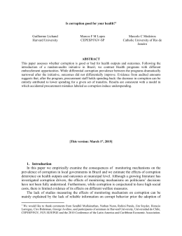
Financial and Economic Development Nexus:
evidence from Brazilian municipalities
Marcos Soares da Silva
September, 2015
399
ISSN 1518-3548
CGC 00.038.166/0001-05
Working Paper Series
Brasília
n. 399
September
2015
p. 1-22
Working Paper Series
Edited by Research Department (Depep) – E-mail: [email protected]
Editor: Francisco Marcos Rodrigues Figueiredo – E-mail: [email protected]
Editorial Assistant: Jane Sofia Moita – E-mail: [email protected]
Head of Research Department: Eduardo José Araújo Lima – E-mail: [email protected]
The Banco Central do Brasil Working Papers are all evaluated in double blind referee process.
Reproduction is permitted only if source is stated as follows: Working Paper n. 399.
Authorized by Luiz Awazu Pereira da Silva, Deputy Governor for Economic Policy.
General Control of Publications
Banco Central do Brasil
Comun/Dipiv/Coivi
SBS – Quadra 3 – Bloco B – Edifício-Sede – 14º andar
Caixa Postal 8.670
70074-900 Brasília – DF – Brazil
Phones: +55 (61) 3414-3710 and 3414-3565
Fax: +55 (61) 3414-1898
E-mail: [email protected]
The views expressed in this work are those of the authors and do not necessarily reflect those of the Banco Central or
its members.
Although these Working Papers often represent preliminary work, citation of source is required when used or reproduced.
As opiniões expressas neste trabalho são exclusivamente do(s) autor(es) e não refletem, necessariamente, a visão do Banco
Central do Brasil.
Ainda que este artigo represente trabalho preliminar, é requerida a citação da fonte, mesmo quando reproduzido parcialmente.
Citizen Service Division
Banco Central do Brasil
Deati/Diate
SBS – Quadra 3 – Bloco B – Edifício-Sede – 2º subsolo
70074-900 Brasília – DF – Brazil
Toll Free: 0800 9792345
Fax: +55 (61) 3414-2553
Internet: <http//www.bcb.gov.br/?CONTACTUS>
Financial and Economic Development Nexus: evidence
from Brazilian municipalities*
Marcos Soares da Silva**
Abstract
The Working Papers should not be reported as representing the views of the Banco Central do
Brasil. The views expressed in the papers are those of the author(s) and do not necessarily reflect
those of the Banco Central do Brasil.
This paper investigates the relationship between financial development and
economic development for 5,564 Brazilian municipalities in 2012. Using supply-side
information, we propose a way to measure financial development at the municipality
level. This composite index is used to evaluate how financial service is distributed
throughout the country. Our empirical strategy consists in examining the effect of
spatial dependence among municipalities by applying a spatial-autoregressive with
spatial-autoregressive disturbance model (SARAR). We find a positive and
significant association of the economic development between the municipality and
its neighbors, after controlling for relevant factors. The results also suggest that
financial development has a large positive impact on local economic development.
JEL Classification: C31, E44, O16, R12
Keywords: Financial development, economic development, cross-sectional spatial
models, economic geography.
*
The author wish to thanks anonymous reviewers for their suggestions, which have helped improve the
paper.
**
Research Department, Banco Central do Brasil. E-mail: [email protected]
3
1.
Introduction
Financial development undoubtedly plays a constructive role in economic development,
largely by improving the quality of financial infrastructure and, to a lesser degree by
raising the quality of socioeconomic infrastructure in its wider sense. The presence of
banks in a region eases access to sophisticated financial marketplaces. The theoretical
connection between financial services and economic prosperity operates through different
channels that facilitate the screening and monitoring of investment projects. First, an
efficient financial system can adequately mobilize savings and allocate resources by
choosing safe and profitable projects (Greenwood et al., 2010). Thus, financial
institutions distribute resources from low-growth to modern high-profitable economic
sectors. Furthermore, they encourage an entrepreneurial response in these dynamic
economic sectors. Second, banks may contribute to reducing agency costs, encouraging
innovation and diversification of economic activities (Aghion et al., 2005). Third, it is
possible to obtain a high rate of return on investments through risk-sharing (Greenwood
and Jovanovic, 1990). Finally, financial institutions provide liquidity to households and
enterprises, smoothing consumption cycles. In this sense, banks follow economic growth
because of the increased demand for financial services (Friedman and Schwarz, 1963).
The theoretical and empirical literature postulates that the association between financial
development and economic development is positive but possibly not monotonic. Indeed,
the effect of financial deepening on growth becomes negative once a certain threshold is
reached (Arcand et al., 2012 and Cecchetti & Kharroubi, 2012). From a cross country
study, Samargandi et al. (2014) find evidence that there is an inverted U-shaped
relationship between financial development and economic growth in the long run. This
may be due to suboptimal low savings, suboptimal high allocation of labor to the financial
sector, overheated economic capacity, or the exertion of inefficiently high cost on the
economy (Jappelli and Pagano, 1994; Bolton et al., 2011; Zeira, 1999; Santomero and
Seater, 2000). Also, Allen and Carlett (2006) e Gai et al.(2008) claim that financial
development may lead to higher systemic risk.
Even though there is an extensive empirical literature available on the relationship
between financial development and economic development, the mainstream literature
uses datasets with high levels of aggregation. As such spatial dependence is not
considered. For example, Ductor and Grechyna (2015) evaluate that link by using a panel
4
data for developed and developing countries. Moreover, only a few studies, as Crocco et
al. (2009) consider spatial dependence.
However, no work has so far focused on financial development as a multidimensional
phenomenon that includes both use and availability of a large range of financial services
across municipalities in Brazil. Hence, in this paper we take into account geographic
space when analyzing the interactions between economic and financial development. We
also investigate which Brazilian municipalities’ features can strengthen the linkages
between financial services and local economic development.
The main purpose of this article is to evaluate whether there is a spatial interdependence
between economic development and financial development at a municipal level in Brazil.
We use a dataset maintained by the Central Bank of Brazil that contain detailed
information on the access to bank services at the municipal level. These data are joined
with the gross domestic product of the municipalities. We also consider a countrywide
level survey carried out by the Brazilian Institute of Geography and Statistics (IBGE),
which provides information on the economic profile of all the Brazilian municipalities in
2012. Our empirical strategy consists in examining the effect of the spatial dependence
among municipalities by applying a spatial-autoregressive with spatial-autoregressive
disturbance model (SARAR). See Kelejian and Prucha (1998, 2010) and Drukker et al.
(2013).
After controlling for relevant factors, we find a positive and stable correlation between
financial development and economic development. In addition, the results suggest that
there may be spillover benefits from dynamic municipalities toward their neighbors.
The remainder of this paper is structured as follows. Section 2 provides statistics for the
financial sector in Brazil. The empirical strategy is explained in Sections 3 and 4. In
Section 5, we discuss the results. In Section 6, conclusions are drawn.
2.
Brazilian financial development
Brazil has experienced strong growth of the banking sector in recent years, accompanied
by a process of restructuring and modernization of the banking industry. The total
financial system credit operations reached R$3,026.4 billion in February 2015, and the
credit/GDP ratio increased to 58.6% from 22.5% in 2002.
5
The regional credit allocation appears to be quite similar to the spatial distribution of
national income. The Southeast region, the most developed, represents 55.0% of the GDP
and has 55.4% of the credit. The South region's share of credit is 18.1%, which is slightly
higher than its share of GDP (16.0%). The northeastern participation in credit accounts
for 13.1%, that is slightly below its share of GDP (13.4%). The Midwest has a bit more
credit (10.5%) than its share of GDP (9.6%). Finally, the North region’s credit share is
3.8%, representing 5.4% of GDP. These figures suggest that there is low interregional
savings mobility in the country.
To understand the access to financial services in Brazil, first, it is important to know how
the channels are distributed in the territory. Table 1 shows the main financial service
channels by region.
Table 1. Financial services distribution channels
PAB Other channels*
Region
Bank branches
PAE Correspondents
Midwest
1,851
3,850
6,546
466
321
North
1,053
2,614
4,284
396
288
Northeast
3,759
8,030
25,289
785
1,178
Southeast
12,112
18,611
34,307
3,454
1,623
South
4,376
7,249
10,430
1.344
555
Brazil
23,151
40,354
80,856
6,445
3,965
Sources: BCB/Unicad
Note: (*) Credit Unions, Cooperative Service Outposts (PAC), and Advanced Service Outposts (PAA).
Correspondents1 are the dominant financial service channel in Brazil, with more than 80
thousand units (52.2% of all distribution channels), followed by Electronic Service
Outposts (PAE2) with 26.1% and bank branches (15.0%). All of these channels have a
strong presence in the Southeast, with 52.3% of bank branches, 42.4% of correspondents
and 46.1% of PAE, respectively, located in this region. Brazil’s correspondent model has
become a well-established alternative approach to increasing access to financial services
and serves as an important instrument for democratizing the delivery and use of these
services. Bank Service Outposts (PAB), which is usually installed inside a government
agency or private company, is a satellite of a bank that can provide all of the services the
financial institution is authorized to run.
1 In this channel, financial institutions hire retailing shops, lottery outlets, post offices, to use them as their
agents, known as correspondents. The correspondents carry out diverse financial transactions on the behalf
of the hiring financial institution.
2 PAEs offer services exclusively through Automated Teller Machines (ATMs).
6
In terms of geographical distribution, the country has an average of 2.33 branches per
1,000 km2. However, this diverges considerably between the five regions. The Southeast
region has approximately five times more branches per 1,000 km² than the national
average, while the North and Midwest barely have one branch per 1,000 km2. The size
and low population density of these regions explain these low levels, particularly in the
North.
The indicator “number of bank branches per 10,000 adults” reveals that the North region
(with 0.9) is 22% below the national average (1.2). The Northeast region, which has
higher population density, is equally low (30.9% below the national average). In contrast,
the South has the highest rate (58.1% higher than the national average), followed by the
Southeast (35.9%) and the Midwest (31.1%).
Although Brazil is above average among developing countries in terms of number of
branches per 100,000 adults (27.7), it falls short when compared to developed countries,
even when only the Southeast or South Brazilian regions are considered.
3.
Analytical framework
Using supply-side information, we calculate a financial development index at the
municipality level. Given the availability of data, the following twelve indicators are
considered:
a)
Geographic penetration:

number of bank branches per thousand kilometer area;

number of Electronic Service Outposts (PAE) per thousand kilometer area;

number of bank services outposts per kilometer area;

number of “advanced service outposts” per kilometer area;

number of “correspondents” per kilometer area;
b)
Demographic penetration:

number of bank branches per 100 thousand people;

number of Electronic Service Outposts (PAE) per 100 thousand people;

number of bank services outposts per 100 thousand people;

number of “advanced service outposts” per 100 thousand people;

number of “correspondents” per 100 thousand people;
c)
Financial service usage:
7

deposit-GDP ratio;

credit-GDP ratio.
The normalized variable is therefore bounded between 0 and 1, where the maximum score
is attributed to the leading municipality in each considered dimension, which is given by:
𝑍𝑘,𝑖 =
(𝑋𝑘,𝑖 − 𝑚𝑘 )
(1)
(𝑀𝑘 − 𝑚𝑘 )
where 𝑋𝑘,𝑖 is the k-th indicator for the i-th municipality. 𝑀𝑘 and 𝑚𝑘 are the maximum
and the minimum values of each financial indicator, respectively.
We then use factorial analysis (principal-component method) to group the financial
indicators into relevant dimensions. It reduces the number of variables in the analysis by
describing linear combinations of them that contain most of the information and
meaningful interpretations.
As shown in Table 2 below, it is enough to retain the first four factors because they capture
almost all of the variance involved in the original dataset.
Table 2. Factor analysis
Factor
Factor 1
Factor 2
Factor 3
Factor 4
Source: Author
Eigenvalue
4.6348
1.9068
1.1106
0.5508
Difference
2.7281
0.7962
0.6098
0.1372
Proportion
0.5663
0.2330
0.1357
0.0612
Cumulative
0.5663
0.7993
0.9349
0.9961
Table 3 shows orthogonal rotated factor loadings (pattern matrix) and unique variances.
Although the first three factors can explain more than 93% of the variance, the fourth
factor is required in order to avoid misrepresentation of the variables “Number of
PAE/Adult Population” and “Number of Correspondent/Adult Population”.
8
Table 3. Factor analysis and unique variances
Variable
# of bank branches/Km2
# of PAE/Km2
# of BSO/Km2
# of ASP/Km2
# of Corresp/Km2
# of Branches/Adult Pop
# of PAE/Adult Pop
# of BSO/Adult Pop
# of ASP/Adult Pop
# Corresp/Adult Pop
Deposit/GDP ratio
Credit/GDP ratio
Source: Author
Factor1
0.8518
0.8333
0.8647
0.7633
0.8420
0.3025
0.2106
0.6855
0.6492
0.1003
0.4078
0.3699
Factor 2
0.2268
-0.0206
-0.2462
-0.4080
0.0055
0.7153
-0.0201
-0.2749
-0.4388
0.1131
0.7598
0.7673
Factor 3
-0.3635
-0.4741
-0.0063
0.3276
-0.4709
0.2768
-0.0596
0.4149
0.5043
0.0064
0.1871
0.2616
Factor 4
-0.1053
0.0887
-0.1145
-0.0004
-0.0965
0.1416
0.8129
-0.0410
0.0417
0.6022
-0.1339
-0.0605
Uniqueness
0.0797
0.0725
0.1786
0.1435
0.0599
0.3003
0.2908
0.2807
0.1299
0.6145
0.2035
0.2024
To obtain the final score, we consider the weights proportionally to the extracted factors,
i.e., factor 1 (0.57), factor 2 (0.23), factor 3 (0.14) and factor 4 (0.06). Thus, the composite
index is a proxy for our financial development measure. It involves the dimensions of
geographic penetration, population coverage and access to financial services both directly
via bank branch and by outreach mechanisms used by the financial institutions.
Table 4 presents the distribution of the “Financial Development Index” by region. These
figures reveal considerable imbalance between regions as a natural consequence of the
diverse socioeconomic conditions that have determinant impacts on the distribution of
financial services. Figure 1 details the distribution of financial services by municipalities,
highlighting the strong presence of banks in the Southeast and the South regions, and in
some big cities throughout the country3.
Table 4. Summary statistics of Financial Development by region
Statistics
Minimum
Maximum
Mean
Std. Dev.
10-percentile
25-percentile
50-percentile
75-percentile
90-percentile
Source: Author
Brazil
0.00
0.98
0.25
0.15
0.10
0.14
0.21
0.31
0.43
North
0.00
0.79
0.16
0.08
0.09
0.11
0.14
0.20
0.26
3
Northeast
0.00
0.86
0.18
0.10
0.10
0.12
0.16
0.22
0.28
Midwest
0.00
0.90
0.22
0.10
0.12
0.15
0.20
0.26
0.32
Southeast
0.00
0.91
0.31
0.17
0.14
0.20
0.28
0.39
0.50
South
0.00
0.98
0.30
0.16
0.12
0.19
0.29
0.37
0.51
We divided the sorted data into ten equal parts so that each interval represents the 10th, 20th, 30th, 40th,
50th, 60th, 70th, 80th, and 90th percentiles of the variable Financial Development Index.
9
Figure 1. Financial Development Index – Spatial Distribution among Brazilian Municipalities in 2012
Source: Author
4.
Empirical specification and data
We are interested in investigating how financial development can contribute to enhancing
economic progress. Our central hypothesis is that credit supply is only effective in
locations where there exist favorable conditions for establishing productive activities.
Moreover, we suppose that there may be spillover benefits across geographical areas.
We follow Kelejian and Prucha (1998, 2010), and the references cited therein, as well as
Drukker et al. (2013), and employ the following econometric model, which allows for
cross-unit interactions:
𝑌𝑖 = 𝜆 ∑𝑛𝑗=1 𝑤𝑖𝑗 𝑌𝑗 + 𝛽0 𝑋𝑖 + 𝛽𝑘 ∑𝑘𝑙=1 𝑍𝑖 + 𝛼 + 𝑢𝑖
(2a)
𝑢𝑖 = 𝜌 ∑𝑛𝑗=1 𝑚𝑖𝑗 𝑢𝑗 + 𝜀𝑖
(2b)
10
where 𝑌𝑖 is an (𝑛 × 1) vector of observations that represents the Economic Development
Index for each Brazilian municipality. 𝑤𝑖𝑗 and 𝑚𝑖𝑗 are (𝑛 × 𝑛) spatial-weighting
matrices (with zero diagonal elements). 𝑤𝑖𝑗 𝑌𝑗 and 𝑚𝑖𝑗 𝑢𝑗 are (𝑛 × 1) vectors referred to
as spatial lags4. 𝜆 and 𝜌 are the corresponding scalar parameters. 𝑋𝑖 and 𝑍𝑖 are (𝑛 × 𝑘)
matrices of explanatory and control variables, respectively. 𝜀𝑖 is an (𝑛 × 1) vector of
innovations, where 𝜀𝑖 ~ 𝑁(0, 𝜎𝜀2 𝐼𝑛 ), and 𝑛 is the sample size.
In this model, the spatial dependence occurs via the error term and the dependent variable
so that a shock in any location is transmitted to the remainder of the locations.
Following the United Nations Development Program’s methodology, we calculate 𝑌𝑖 ,
“Municipal Economic Development Index”, as follows:
[𝑙𝑛(𝐺𝐷𝑃𝑖𝑃𝐶 ) − 𝑙𝑛(𝑀𝑖𝑛𝑅𝑒𝑓)]
𝑌𝑖 = [𝑙𝑛(𝑀𝑎𝑥𝑅𝑒𝑓)
(3)
− 𝑙𝑛(𝑀𝑖𝑛𝑅𝑒𝑓)]
where 𝐺𝐷𝑃𝑖𝑃𝐶 is the monthly gross domestic product per capita at a given municipality.
MaxRef and MinRef are the maximum and the minimum reference values defined as
R$8.00 and R$4,033.00, respectively. The later value corresponds to the average income
of the richest decile of the population in the richest municipality in Brazil while the former
value corresponds to approximately $100 purchasing power parity (PPP), which is the
adopted limit for calculating the Human Development Index (HDI) by the United Nations
Development Programme.
The variable explanatory 𝑋𝑖 denotes the Financial Development Index for each
municipality as discussed in Section 4. Theoretically, it is expected to be positively related
to the Economic Development Index.
Control variables do not solely help us to account for spurious relationships, but they also
measure the impact of any given variable above and beyond the effects of other variables.
For controlling and gaining insight in whether a municipality is economic developed, we
use the variable described below. To this end, we use a nationwide level survey covering
all the Brazilian municipalities carried out by the Brazilian Institute of Geography and
Statistics.
4
In this study, 𝑤𝑖𝑗 and 𝑚𝑖𝑗 are identical matrices.
11
We define the hierarchy of municipalities and delimit the regions of influence associated
with them from the aspects of public administration and corporate management and the
provision of equipment and services. This is performed in order to identify points of the
territory from which decisions are issued. In this study, we categorize the municipalities
into four groups, depending on how easily they can reach each other. Hence, we have the
following dummies variables: 1) Centrality Level 1 (national): municipality whose
leadership transposes all regions of the country; 2) Centrality Level 2 (regional):
municipality that exerts influence over other municipalities within its administrative
region; 3) Centrality Level 3 (subregional): municipality whose linkages are bounded by
others within the same mesoregion; 4) Centrality Level 4 (local): municipality that is
linked only to its nearest neighbors or that it does not have connections. The primary
reason for the lack of connection is the existence of a business relationship purely for
local purposes. In spatial terms, the locations of disconnected municipalities are scattered
throughout Brazil.
Besides the degree of centrality, we can also ask questions about the correlation pattern
in the degrees of connected municipalities. Therefore, we use one measure of connection
called Linkage Intensity, which comprises the sum of companies and branches
circumscribed by each symmetrical pair of municipalities.
We also include as covariate the variable Average Interaction Path, which shows the
average distance between municipalities that have economic connection. The average
distance of the interactions between the municipalities is 395 km. São Paulo (815 km),
Rio de Janeiro (950 km), and Brasilia (1,062 km) express the extent of its dense network
fed by the condition of national metropolis. According to IBGE, more than half of the
population in Brazil lives in towns that form clusters of economic conglomerates.
Broadly speaking, a suitable transport infrastructure can promote business activities and
reduce the commuting cost, improving the economic conditions. We include as a control
the variable Public Transport. This covariate is a dummy variable that assumes the value
of one if there is regular public transportation that meets displacement between
neighborhoods, districts and other localities of the municipality, and zero otherwise.
The dummy variable Investment Policy takes on the value of one if the municipality
offers incentives to attract productive investments, and zero otherwise.
12
The strength of linkages between two municipalities is evaluated by the interactions
among local and non-local establishments. In this evaluation, we take into account the
presence of branches that are attracted to their domains. This process is captured by the
explanatory variable Attracted Business, which represents the number of firms or
branches whose head office is not located in the municipality of reference.
Remote access refers to financial services accessed by personal devices, such as landline
or cell telephones and personal computers. These kinds of services may include call
centers, internet banking, and mobile banking. Thus, it vital to narrow the digital gap in
the municipalities poorly served with regular financial services. We try to capture this
dimension by using the dummy variable Digital Inclusion, whose value is one if the
municipality develops actions in order to induce digital inclusion, and zero otherwise.
Finally, the variable Linkage Intensity represents the degree to which a municipality
does business with other municipalities. It is gauged by the sum of the number of local
companies that maintain affiliated units in other localities and the number of firms
attracted (or branches) to the municipality as well.
While the availability of financial services contributes to raising the local economy, banks
may prefer establishing their financial services where income is already higher. This
reverse effect could lead to an endogeneity problem in the model specification of
Equation 2.
We instrument our financial development index with two instrumental variables. First,
the average employed population ratio of the neighboring municipalities in the same
economic microregion, excluding the municipality of reference. Second, the payroll of
local firm-related employees located outside the municipality. As banks fund productive
projects, these variables are expected to be strongly correlated with finance activities. In
addition, it is reasonable to consider that the employed population that commutes is
negligible as the distance increases due to transportation costs. Consequently, such
instrumental variable is not likely to affect the income in the municipality of reference.
We use the Hansen J over-identification test of all the instruments to check their validity.
5.
Regression results
The main purpose of this article is to evaluate whether there is a spatial interdependence
between economic development and financial development at a municipal level in Brazil.
13
This study provides several interesting findings in relation to the role that spatial
interdependence plays as a determinant of local economic development. Tables 5 reports
the main results of spatial-autoregressive model with spatial-autoregressive disturbances,
considering a contiguity matrix of neighborhood. We calculated robust standard errors
for robust estimators, where the standard error estimates are designed to be robust against
heteroskedasticity and the presence of outliers.
As a robustness test, we also run the regression with two different criteria of
neighborhood. One model specification were carried out including a second order
neighboring, considering the inverse distance weighting matrix and the cut-off of 80 km
(Table 6), while another extends this criterion to 200 kilometers (Table 7). The results are
similar to our benchmark specification. Nevertheless, spatial effects are considerably
higher when the first order contiguity matrix is taken into account. In addition, as shown
in Table 8, where we do not take into account spatial dependence, neither related to the
term error nor the dependent variable lag, the correlation between financial development
and economic development seems to be overestimated by the two-stage least squares
estimator.
The robust Durbin-Wu-Hausman test of endogeneity leads to a strong rejection of the null
hypothesis that the variable Financial Development Index is exogenous. This confirms
the need for using instrumental variable estimators. In contrast, the Hansen’s test does not
reject the null hypothesis that all of the aforementioned instruments are valid, confirming
that they are indeed exogenous.
14
Table 5. Estimation results for the Spatial-autoregressive model with spatial-autoregressive disturbances
(matrix – bordering neighbors).
Variable
Specification 1
Specification 2
Specification 3
Spatial Dependence Lag
0.2479***
(0.0465)
0.2581***
(0.0611)
0.1909***
(0.0540)
Financial Development Index
0.3696***
(0.0289)
0.3745***
(0.0366)
0.4072***
(0.0354)
North Region
-0.0146***
(0.0046)
-0.0098**
(0.0354)
-0.0152***
(0.0047)
South Region
0.0273***
(0.0030)
0.0254***
(0.0029)
0.0273***
(0.0031)
Northeast Region
-0.0399***
(0.0044)
-0.0372***
(0.0047)
-0.0429***
(0.0044)
Midwest Region
0.0359***
(0.0033)
0.0368***
(0.0041)
0.0380***
(0.0042)
Centrality Level 2
0.0738***
(0.0217)
0.0731***
(0.0243)
Centrality Level 3
0.0482**
(0.0194)
0.0479**
(0.0354)
Centrality Level 4
0.0742***
(0.0252)
0.0774***
(0.0269)
Public Transport
0.0101***
(0.0022)
0.0094***
(0.0022)
Investment Policy
0.0059***
(0.0014)
0.0051***
(0.0014)
Digital Inclusion
0.0087***
(0.0026)
0.0089***
(0.0026)
Attracted Business
-0.3355
(0.2055)
Average Interaction Path
0.0233***
(0.0070)
Linkage Intensity
0.3893***
(0.1951)
Constant
0.3950***
(0.0565)
0.2949***
(0.0611)
0.3280***
(0.0335)
Rho
0.3105***
(0.0357)
0.2275***
(0.0455)
0.2821***
(0.0335)
Wald Test
482.23
(0.0000)
1,553.73
(0.0000)
1,539.19
(0.0000)
Durbin-Wu-Hausman
(test of endogeneity)
189.03
(0.0000)
170,66
(0.0000)
114.7700
(0.0000)
Hansen (p-value)
(0.4058)
(0.4710)
(0.8630)
5,564
5,564
5,564
0.7045
0.7213
0.7683
Observation
2
R -Adjusted
Note: Robust standard errors reported in parentheses. ***, **, and * indicate significance at the 1%, 5%,
and 10%, respectively. The Hansen test evaluates the validity of the over-identifying restrictions.
Specification 1 is a restricted econometric model in which we include as explanatory variables only the
Financial Development Index, the spatial-autoregressive and the spatial-autoregressive disturbance term.
Specification 2 adds categorical variables that characterize the economic profile of the Brazilian
municipalities. Specification 3 is an extended model in which we include as regressors other similar
variables that are measured at the ratio level.
15
The results indicate a significant and positive association between economic development
in a municipality and its neighbors, after controlling for relevant factors. This means that
spatial relationship across municipalities is somewhat relevant. The economic progress
of the municipality is indeed affected by the performance of its neighbors, and therefore
it is influenced by its geographic position. These findings also suggest that the spillover
effects among municipalities are essential to economic growth, so that municipalities can
gain from increased economic activity in their neighboring municipalities.
As theoretically expected, we find that financial development has a positive and high
significant impact on economic development, which suggests that the financial
infrastructure that there is both inside and around the municipality matters, in the sense
that it can be useful to those communities that do not have such services. This is in line
with earlier studies. Research conducted by Raj et al. (2014) has shown that local bank
availability is associated with significant increase in enterprises in the informal sector in
India. Samargandi et al. (2014) and Ductor and Grechyna (2015) have found empirical
evidence in favor of the existence of an optimal level of financial development given by
the characteristics of an economy.
The results also confirm that municipalities that establish and develop mechanisms for
supporting digital inclusion program are better off than those that do not have any action
in this regard. This kind of program provides the ordinary people the skills of modern
technology so that they can be reached by strategy adopted by the Brazilian financial
institutions, which has been rapidly expanding their banking services through alternative
mechanism to traditional bank branch. Indeed, branchless banking services have become
widely spread in Brazil. For instance, correspondent banking is present in 93.2% of the
Brazilian municipalities, including 1,761 out of 1,932 of those without any bank branch.
Lack of proper public transport can constrain the access to goods and services,
particularly in regions where traveling or commuting can be proved extremely lengthy
and time-consuming. As a result, it may be an important barrier to financial inclusion in
areas sparsely inhabited. Therefore, it is not a surprise that the proxy for public transport
services is positively related to economic development.
We find a significant positive association between economic development and the active
municipal investment policy implemented to attract new business. This result suggests
that, for instance, if one municipality reduces local tax or provides support to
16
entrepreneurship, in order to encourage new enterprises, it will have relative advantages
over its neighbors.
Overall, this study reveals that centrality is important. Therefore, the municipalities that
are well located in the network of business relationships have advantages compared to
those disconnected or located in peripheral positions. However, we find that local
connections are also relevant to economic development, strengthening national and
interregional connections.
6.
Concluding remarks
In this study, we have tested whether financial development affects economic
development. The usual way to do this is to investigating how the availability and usage
of financial service are associated with economic progress. By estimating a generalized
spatial autoregressive model, we also investigated whether improvements in one
municipality will have a spillover effect on its neighboring areas.
We obtained several insightful results. First, the results point to a positive spatial
association among municipalities in Brazil. This fact suggests that a developed locality
tends to be surrounded by other municipalities that are similarly developed. Likewise,
poor regions are connected with undeveloped areas. Second, we find that the municipal
financial infrastructure is highly related to the level of local economic development.
Finally, from a policy perspective, our findings indicate that economic development can
be encouraged by local policy-makers.
This article hopes to bring into the debate the importance of geographical location for
studies on financial development. Further research might analyze financial inclusion and
focus attention on particular regional areas. Besides, it would be interesting to use
network measurement to analyze the topology of the banking network across the country.
17
Reference
Aghion, P.; Howit, P.; Mayer-Foulkes, D. (2005). The effect of financial development on
convergence: theory and evidence. The Quarterly Journal of Economics, 120(1), 173222.
Allen, F. Carletti, E (2006). Credit risk transfer and contagion. Journal of Monetary
Economics, 53(1), 89-111.
Arcand, J., Berkes, E., & Panizza, U. (2012). Too much finance? International Monetary
Fund, Research Department.
Bencivenga, V.R.; Smith, B.D. (1991). Financial intermediation and endogenous growth.
The Review of Economic Studies, 58(2), 195-209.
Bolton, P.; Santos, T.; Scheinkman, J.A. (2011). Cream skimming in financial markets.
Working Paper, 16804. National Bureau of Economic Research.
Cecchetti, G., & Kharroubi, E. (2012). Reassessing the impact of finance on growth. BIS
Working Paper No. 381. Bank for International Settlements.
Crocco, M.; Santos, F.; Amaral, P. (2009). The spatial structure of the financial
development in Brazil. UFMG-Cedeplar Texto para Discussão, 361.
Drukker, D.M.; Egger, P.; Prucha, I.R. (2013). On two-step estimation of a spatial
autoregressive model with autoregressive disturbances and endogenous regressors.
Econometric Reviews, 32, 686-733.
Ductor, L.; Grechyna, D. (2015). Financial development, real sector, and economic
growth. International Review of Economics and Finance. In Press: available online 13
January 2015.
Friedman, M.; Schwartz, A. (1963). A Monetary history of the United States. Princeton:
Princeton University Press.
Gai, P.K.; Millard, S.; Perez, A. (2008). Financial innovation, macroeconomic stability
and systemic crises. The Economic Journal, 111(527), 401-426.
Greenwood, J.; Jovanovic, B. (1990). Financial development, growth, and the distribution
of income. Journal of Political Economy, 98(5), 1076-1107.
Greenwood, J.; Sanchez, J.; Wang, Ch. (2010). Financing development: the role of
information costs. The American Economic Review, 100, 1875-1891.
Instituto Brasileiro de Geografia e Estatística (2012). Relatório de Gestão do Território.
Jappelli, T; Pagano, M. (1994). Saving, growth, and liquidity constraints. The Quarterly
Journal of Economics, 109(1), 83-109.
Kelejian, H.H.; Prucha, I.R. (1998). A generalized spatial two-stage least squares
procedure for estimating a spatial autogressive model with autoregressive disturbances.
Journal of Real Estate Finance and Economics, 17, 99-121.
Kelejian, H.H.; Prucha, I.R. (2010). Specification and estimation of spatial autoregressive
models with autoregressive and heteroskedastic disturbances. Journal of Econometrics,
157, 53-67.
18
Raj, S.N.R.; Sen, K.; Kathuria, V. (2014). Does banking development matter for new firm
creation in the informal sector? Evidence from India. Review of Development Finance, 4,
38-49.
Samargandi, N.; Fidrmuc, J.; Ghosh, S. (2014). Is the relationship between financial
development and economic growth monotonic? Evidence from a sample of middleincome countries. World Development, 68, 66-81.
Santomero, A.M.; Seater, J. J. (2000). Is there an optimal size for the financial sector?
Journal of Banking and Finance, 24(6), 945-965.
Zeira, J. (1999). Informational overshooting, booms, and crashes. Journal of Monetary
Economics, 43(1), 237-257.
19
Table 6. Estimation results for the Spatial-autoregressive model with spatial-autoregressive
disturbances (matrix - inverse distance with 80 kilometers cut off)
Variable
Spatial Dependence Lag
Financial Development Index
North Region
South Region
Northeast Region
Midwest Region
Specification 4
0.0157***
(0.0042)
0.4184***
(0.0192)
-0.0236***
(0.0047)
0.0177***
(0.0057)
-0.0645***
(0.0037)
0.0484***
(0.0039)
Specification 5
0.0081**
(0.0038)
0.4490***
(0.0325)
-0.0225***
(0.0049)
0.0177***
(0.0052)
-0.0337***
(0.0037)
0.0454***
(0.0037)
0.0874***
(0.0205)
0.0721***
(0.0186)
0.0976***
(0.0233)
0.0114***
(0.0021)
0.0060***
(0.0014)
0.0073***
(0.0026)
0.5442***
(0.0060)
0.6929***
(0.0287)
3,481.37
(0.0000)
135.57
(0.0000)
(0.3615)
0.4282***
(0.0314)
0.6870***
(0.0038)
5,395.25
(0.0000)
29.31
(0.0095)
(0.4478)
Specification 6
0.0082**
(0.0041)
0.4523***
(0.0326)
-0.0261***
(0.0050)
0.0173***
(0.0052)
-0.0651***
(0.0037)
0.0337***
(0.0038)
0.0769***
(0.0237)
0.0622**
(0.0218)
0.0873***
(0.0259)
0.0110***
(0.0022)
0.0057***
(0.0015)
0.0078***
(0.0027)
-0.3890**
(0.1987)
0.0217***
(0.0072)
0.4341**
(0.1849)
0.4364***
(0.0328)
0.6889***
(0.0328)
4,478.77
(0.0000)
150.23
(0.0000)
(0.6235)
5,564
0.7021
5,564
0.7418
5,564
0.7392
Centrality Level 2
Centrality Level 3
Centrality Level 4
Public Transport
Investment Policy
Digital Inclusion
Attracted Business
Average Interaction Path
Linkage Intensity
Constant
Rho
Wald Test
Durbin-Wu-Hausman
(test of endogeneity)
Hansen (p-value)
(test of overidentification)
Observation
R2-Adjusted
Note: Robust standard errors reported in parentheses. ***, **, and * indicate significance at the 1%, 5%,
and 10%, respectively. The Hansen test evaluates the validity of the over-identifying restrictions.
Specification 4 is a restricted econometric model in which we include as explanatory variables only the
Financial Development Index, the spatial-autoregressive and the spatial-autoregressive disturbance term.
Specification 5 adds categorical variables that characterize the economic profile of the Brazilian
municipalities. Specification 6 is an extended model in which we include as regressors other similar
variables that are measured at the ratio level.
20
Table 7. Estimation results for the Spatial-autoregressive model with spatial-autoregressive
disturbances (matrix - inverse distance with 200 kilometers cut off)
Variable
Spatial Dependence Lag
Financial Development Index
North Region
South Region
Northeast Region
Midwest Region
Specification 7
0.0096***
(0.0021)
0.4026***
(0.0178)
-0.0245***
(0.0054)
0.0003***
(0.0055)
-0.0633***
(0.0040)
0.0472***
(0.0067)
Specification 8
0.0056**
(0.0019)
0.4339***
(0.0315)
-0.0201***
(0.0054)
0.0235***
(0.0050)
-0.0585***
(0.0040)
0.0478***
(0.0043)
0.0841***
(0.0207)
0.0662***
(0.0186)
0.0925***
(0.0235)
0.0117***
(0.0021)
0.0064***
(0.0014)
0.0065***
(0.0026)
0.5462***
(0.0067)
0.4289***
(0.0174)
3,076.69
(0.0000)
173.74
(0.0000)
(0.3471)
0.4321***
(0.0319)
0.4304***
(0.0209)
3,855.37
(0.0000)
215.68
(0.0000)
(0.4613)
Specification 9
0.0062**
(0.0021)
0.4322***
(0.0305)
-0.0241***
(0.0054)
0.0229***
(0.0050)
-0.0601***
(0.0039)
0.0460***
(0.0043)
0.0737***
(0.0239)
0.0563**
(0.0218)
0.0821***
(0.0260)
0.0113***
(0.0022)
0.0060***
(0.0014)
0.0070***
(0.0026)
-0.3495*
(0.1915)
0.0259***
(0.0071)
0.3787*
(0.1849)
0.4405***
(0.0020)
0.4316***
(0.0207)
4,042.04
(0.0000)
760.41
(0.0000)
(0.6681)
5,564
0.6681
5,564
0.6913
5,564
0.7292
Centrality Level 2
Centrality Level 3
Centrality Level 4
Public Transport
Investment Policy
Digital Inclusion
Attracted Business
Average Interaction Path
Linkage Intensity
Constant
Rho
Wald Test
Durbin-Wu-Hausman
(test of endogeneity)
Hansen (p-value)
(test of overidentification)
Observation
R2-Adjusted
Note: Robust standard errors reported in parentheses. ***, **, and * indicate significance at the 1%, 5%,
and 10%, respectively. The Hansen test evaluates the validity of the over-identifying restrictions.
Specification 7 is a restricted econometric model in which we include as explanatory variables only the
Financial Development Index, the spatial-autoregressive and the spatial-autoregressive disturbance term.
Specification 8 adds categorical variables that characterize the economic profile of the Brazilian
municipalities. Specification 9 is an extended model in which we include as regressors other similar
variables that are measured at the ratio level.
21
Table 8. Estimation results for the Linear Instrumental-Variables Regression
Variable
Financial Development Index
North Region
South Region
Northeast Region
Midwest Region
Specification 10
0.4119***
(0.0139)
-0.0277***
(0.0035)
0.0344***
(0.0023)
-0.0643***
(0.0023)
0.0438***
(0.0026)
Specification 11
0.5092***
(0.0187)
-0.0131***
(0.0038)
0.0325***
(0.0021)
-0.0531***
(0.0028)
0.0504***
(0.0032)
0.1121***
(0.0084)
0.0722***
(0.0073)
0.1271***
(0.0094)
0.0093***
(0.0022)
0.0065***
(0.0017)
0.0085***
(0.0025)
0.5506***
(0.0044)
11,293.38
(0.0000)
454.13
(0.0000)
(0.37141)
0.3828***
(0.0133)
8,928.21
(0.0000)
532.65
(0.0000)
(0.4406)
Specification 12
0.5134***
(0.0262)
-0.0110**
(0.0046)
0.0302***
(0.0046)
-0.0511***
(0.0032)
0.0525***
(0.0038)
0.0787***
(0.0087)
0.0419***
(0.0079)
0.0940***
(0.0089)
0.0090***
(0.0023)
0.0062***
(0.0017)
0.0089***
(0.0026)
-0.9506***
(0.1585)
0.0061
(0.0074)
0.8742***
(0.1676)
0.4082***
(0.0123)
10,119.18
(0.0000)
395.86
(0.0000)
(0.4742)
5,564
0.5119
5,564
0.5464
5,564
0.5690
Centrality Level 2
Centrality Level 3
Centrality Level 4
Public Transport
Investment Policy
Digital Inclusion
Attracted Business
Average Interaction Path
Linkage Intensity
Constant
Wald Test
Durbin-Wu-Hausman
(test of endogeneity)
Hansen (p-value)
(test of overidentification)
Observation
R2-Adjusted
Note: Robust standard errors reported in parentheses. ***, **, and * indicate significance at the 1%, 5%,
and 10%, respectively. The Hansen test evaluates the validity of the over-identifying restrictions.
Specification 10 is a restricted econometric model in which we include as explanatory variables only the
Financial Development Index, the spatial-autoregressive and the spatial-autoregressive disturbance term.
Specification 11 adds categorical variables that characterize the economic profile of the Brazilian
municipalities. Specification 12 is an extended model in which we include as regressors other similar
variables that are measured at the ratio level.
22