TEXTO PARA DISCUSSÃO N° 294
MODELING ECONOMIC GROWTH FUELLED BY
SCIENCE AND TECHNOLOGY
Américo Tristão Bernardes
Ricardo Machado Ruiz
Leonardo Costa Ribeiro
Eduardo da Motta e Albuquerque
Agosto de 2006
Ficha catalográfica
330.34
B519m
2006
Bernardes, Américo Tristão.
Modeling economic growth fuelled by science and
technology / Américo Tristão Bernardes, Ricardo
Machado Ruiz, Leonardo Costa Ribeiro, Eduardo da
Motta
e
Albuquerque
Belo
Horizonte:
UFMG/Cedeplar, 2006. –
24p. (Texto para discussão ; 294)
1. Desenvolvimento econômico 2. Ciência e
desenvolvimento econômico. 3. Tecnologia e
desenvolvimento econômico. I. Ruiz, Ricardo
Machado II. Ribeiro, Leonardo Costa. .III.
Albuquerque, Eduardo da Motta e. IV. Universidade
Federal de Minas Gerais. Centro de Desenvolvimento
e Planejamento Regional. V Título. VI. Série.
CDU
2
UNIVERSIDADE FEDERAL DE MINAS GERAIS
FACULDADE DE CIÊNCIAS ECONÔMICAS
CENTRO DE DESENVOLVIMENTO E PLANEJAMENTO REGIONAL
MODELING ECONOMIC GROWTH FUELLED BY SCIENCE AND TECHNOLOGY*
Américo Tristão Bernardes
Department of Physics, UFOP
Ricardo Machado Ruiz
Department of Economics, UFMG
Leonardo Costa Ribeiro
Department of Physics, UFMG
Eduardo da Motta e Albuquerque
Department of Economics, UFMG
CEDEPLAR/FACE/UFMG
BELO HORIZONTE
2006
*
The Brazilian agencies CNPq and Fapemig partially supported this work. We thank Thais Henriques and Leandro Silva for
research assistance.
3
SUMÁRIO
1. SCIENCE AND TECHNOLOGY FUELLING ECONOMIC GROWTH ......................................... 6
2. THE CORRELATIONS BETWEEN SCIENCE, TECHNOLOGY AND THE WEALTH OF
NATIONS .......................................................................................................................................... 7
3. SIMULATION MODELS OF ECONOMIC GROWTH.................................................................. 10
4. INNOVATION AND IMITATION IN A MULTI-COUNTRY MODEL ....................................... 11
4.1. Country Economic Structure ...................................................................................................... 12
4.1.1. Price and Production ........................................................................................................... 12
4.1.2. Competitiveness .................................................................................................................. 12
4.1.3. Technological Change ......................................................................................................... 13
4.1.4. Income ................................................................................................................................. 13
4.2. Country Demand, Capital and Savings ...................................................................................... 13
4.2.1. Market Share and Demand .................................................................................................. 13
4.2.2. Capital, Inventory and Savings............................................................................................ 14
5. SIMULATIONS AND RESULTS .................................................................................................... 15
5.1. First Simulation: Initial Random GDPs ..................................................................................... 16
5.2. Second Simulation: Three Different Initial GDPs...................................................................... 18
5.3. Third Simulation: Real and Random Values for Population, Scientific and Technological
Production ................................................................................................................................. 19
6. CONCLUSIONS AND AGENDA FOR FURTHER RESEARCH.................................................. 20
REFERENCES...................................................................................................................................... 22
4
ABSTRACT
This paper suggests a simulation model to investigate how science and technology fuel
economic growth. This model is built upon a synthesis of technological capabilities represented by
national innovation systems. This paper gathers data of papers and patents for 183 countries between
1999 and 2003, GDP and population for 2003. These data show a strong correlation between science,
technology and income. Three simulation exercises are performed. Feeding our algorithm with data
for population, patents and scientific papers, we obtain the world income distribution (R=0.99). These
results support our conjecture on the role of science and technology as a source of the wealth of
nations.
Key-words: simulation models, systems of innovation, economic growth.
JEL Classification: O0
RESUMO
Este artigo propõe um modelo de simulação para investigar a contribuição da ciência e da
tecnologia para o crescimento econômico. O ponto de partida são os sistemas nacionais de inovação,
um conceito que sintetiza a capacitação tecnológica das nações. Desta forma, o modelo pode preservar
simplicidade e parcimônia. Os dados coletados (patentes, artigos e PIB e população, para 183 países)
indicam uma forte correlação entre ciência, tecnologia e renda. Três exercícios com simulações são
realizados. A correlação entre o mundo simulado e o mundo real é alta (R=0,99), quando o algoritmo é
alimentado com dados de população, patentes e artigos científicos.
Palavras-chaves: modelos de simulação, sistemas de inovação, crescimento econômico.
Classificação JEL: O0
5
1. SCIENCE AND TECHNOLOGY FUELLING ECONOMIC GROWTH
This paper suggests a simulation model to investigate how science and technology fuel
economic growth. This model is built upon a synthesis of technological capabilities represented by the
concept of national innovation systems, which allows our model to be parsimonious.
What are the theoretical foundations that underline the concept of national systems of
innovation? National innovation system (NSI) is a concept that shows how a complex interplay of
different actors (firms, universities, public labs, governments, financial institutions etc) pushes the
technological development of nations. NSI shows the engine of technological progress at the centre of
the process of economic development.
Innovation system is a concept developed by Freeman (1988), Nelson (1988) and Lundvall
(1988) in a book that is the first organized presentation of the evolutionist approach as a whole (Dosi
et all, 1988). The timing of this presentation is not casual, because for the elaboration of the concept of
NSI previous theoretical clarifications were necessary (and it is not casual that NSI is the part V of the
book). The first round of this elaboration, at large, took place during the 1970s, with the publication of
three pioneering works: Freeman (1974); Rosenberg (1976) and Nelson and Winter (1977). These
works involved a lot of theoretical synthesis and dialogue with previous elaboration.1
This first round of evolutionary elaboration investigated important subjects as the
determinants of technological progress, the role of firms in innovative activities, the microeconomic
foundations of evolutionary thinking (rationality, firms behaviour, the combination of routines, search
and selection as an alternative to equilibrium etc),2 a historical account of technological change,
including the role of science and its complex interplay with technology, the multifarious actors
involved in innovative activities, the role of markets and non-market institutions in innovation, a
typology of innovations, indicating the role of imitation and incremental change and the
multidimensional changes in the centre of the capitalist system; summarized by Freeman’s elaboration
on different historical phases of capitalist development.
The result of this first round of theoretical elaboration is the ground work for an explosion of
empirical, theoretical and comparative studies using the evolutionary elaboration as reference.
Freeman (1994) and Dosi (1997) describe the rich array of subjects worked out by evolutionists after
this first round. Among this elaboration, the concept of NSI is presented.
A second round of theoretical elaboration takes place during the 1980s and the 1990s: the
concept of NSI is presented (Freeman, 1988, Nelson, 1988 and Lundvall, 1988) and is further
developed. Three developments are important and representative. First, Nelson (1993) organizes a
comparative study gathering historical and empirical evidences to deepen the understanding of the
institutional differentiation between 16 countries (involving developed, catching up and nondeveloped countries, Argentine and Brazil among them). Second, Lundvall (1992) organizes a book
that presents conceptual developments related to the concept of NSI, involving subjects as the role of
scientific infrastructure and the financial dimension. Third, Edquist (1997) presents a mix of
theoretical issues and empirical topics, contributing to qualify the NSI issue and opening new research
1
See Nelson and Winter (1982, pp. 33-45) for a summary of “allies and antecedents of evolutionary theory”.
2
Dosi (1988) presents a broad review of this issue.
6
subjects related to innovation systems. The NSI as a synthesis of previous elaboration opened new
room for further advances in the evolutionary approach in general and for a broadening of the concept
of innovation systems.
The third round of evolutionary elaboration on NSIs emphasises new subjects in the research
agenda: the connections between NSIs, economic growth and development, convergence and
divergence in a global arena. Freeman (1995) is representative of this new round, integrating List’s
elaboration to connect the NSI framework with development issues. This round coincides with the
revival of mainstream economics interest on economic growth during the 1990s. Dosi, Freeman &
Fabiani (1994), Fagerberg (1994), and Nelson (1998) are representative of evolutionists’ interventions
in this debate, benefiting from the rich elaboration of the previous two rounds.
Dosi, Freeman & Fabiani point to a central issue to this paper: how the correlation between
technology and GDP increases throughout the 20th century (1994, Tables 9 and 10, pp. 14-15). This
point is easily integrated with other works, as Narin et all (1997) that show the increasing role of
science and technology as sources of economic development.3
This introduction explains why an investigation on the relationship between science,
technology and development may use NSI as a guiding concept. As a synthesis of national
technological capabilities, innovation systems may be a useful source for modeling economic growth
fuelled by science and technology.
This paper’s model is a result of previous work: Bernardes et all (2003) present a discussion
concerning science and technology and less-developed countries, Ruiz et all (2005) initiates our
modeling elaboration, Ribeiro et all (2006a) concludes this elaboration and suggests a first model and
Ribeiro et all (2006b) cluster countries in three different “regimes”, representing different stages of
NSI formation.
2. THE CORRELATIONS BETWEEN SCIENCE, TECHNOLOGY AND THE WEALTH OF
NATIONS
Statistics of patents (a proxy of technological capabilities) and papers (a proxy of scientific
capabilities) summarize the main features of national systems of innovation. Of course, papers are not
a perfect measure of scientific production, and patents are not a perfect measure of technological
innovation. The literature has both used these data and warned about their problems, limitations and
shortcomings (see Möed et all, 2004). Scientific papers, the data collected by the ISI, have various
shortcomings, from language bias to the quality of research performed: there could be important
research for local needs that does not translate in international papers, but only in national publications
not captured by the ISI database.
There is a large literature on the problems of this indicator. Patents, the USPTO data, also
have important shortcomings, from commercial linkages with the US to the quality of the patent:
again, local innovation necessarily is limited to imitation in the initial phases of development, and
imitation or minor adaptations do not qualify for a patent in the USPTO). Therefore, this paper
3
See references on this subject in Bernardes et all (2003).
7
acknowledges these important limitations, and this literature must be kept in mind to qualify the
results discussed in the next sub-sections. Despite these problems, these two datasets appear to provide
useful information for research.
This paper gathers data of papers and patents for 183 countries between 1999 and 2003. The
option for collecting a broader sample of countries includes countries from different stages of
development and allows a comparison between developed and less-developed countries, including the
transitional position of catching up countries. This data set uses the average for the period 1999-2003,
in order to include more countries, mainly those less developed, with very low scientific and/or
technological production.
Fig. 1 shows a three-dimensional plot, where the log10 of the GDP per capita (US$, PPP,
according to the World Bank, for 2003) is plotted against the log10 of the number of articles per
million of inhabitants (A*) and the log10 of the number of patents per million of inhabitants (P*). The
data are an average for the years 1999-2003. Only countries with data available and scores different
from zero are represented.
Figure 1 shows a strong correlation between science, technology and wealth of nations. Table
1 shows a Correlation Matrix between GNP, patents, articles, and population. There are strong
relationships among these variables, which means that there is some system that connects them. Figure
2 shows the projection of these data on the articles-patents plane. Ribeiro et all (2006b) apply a superparamagnetic clustering technique and find three groups of countries. Hence, they suggest there are
three “regimes” that summarizes different levels of development and different types of NSI.
8
TABLE 1
Correlation Matrix
GNP
GNPpc
POP
PATpc
ARTpc
PAT
ART
GNP
1.0000
0.3606
0.2689
0.6578
0.2631
0.9691
0.9869
GNPpc
POP
PATpc
ARTpc
PAT
ART
1.0000
-0.0786
0.6752
0.8053
0.3015
0.3950
1.0000
0.0385
-0.0726
0.1550
0.2804
1.0000
0.7084
0.6577
0.6743
1.0000
0.2037
0.3335
1.0000
0.9380
1.0000
Data Source: ISI, USPTO and World Bank.
These “regimes” say that there are different mechanisms inside NSI. The interactions between
science and technology seem to be operating more fully in the countries of the most developed regime
(regime 3, represented by squares in Figure 2). Conversely, countries in clusters represented by circles
(regime 2) and by triangles (regime 1) lack critical mass in the scientific infrastructure that weakens
(or even blocks) the feedbacks between science and technology that pushes economic growth.
Ribeiro et all (200b) suggest that as the “regimes” changes, the number and the channels of
interactions between scientific infrastructure, technological production and economic growth also
change. As the country evolves, more connections are turned on and more interactions operate. The
highest regime is the case where all connections and interactions are working. As long as the
development takes place, the role of other aspects, e.g. natural resources, in the causation of economic
growth decreases. As a country upgrades its economic position, its economic growth is increasingly
caused by its scientific and technological resources. The feedbacks between them contribute to explain
why the modern economic growth is fuelled by strong scientific and technological capabilities.
9
FIGURE 2
Three Regimes (1999-2003)
Note: Clusters obtained in applying the super-paramagnetic clustering technique. Three main groups are clearly distinguished
in this figure. The triangles represent countries in regime I, circles stand for those in regime II, and squares represent
countries in regime III. Note that a small group of three countries split at the top of the figure. They are Taiwan, Japan, and
the United States. For details, see Ribeiro et all (2006b).
3. SIMULATION MODELS OF ECONOMIC GROWTH
Section 1 explains why NSI summarizes technological capabilities of countries. Section 2
presents data that are reliable proxies of the main features of NSIs and of their general relationship
with economic development. This leads us to the next step of our inquiry: the investigation of the
causal links between science, technology and the wealth of nations. The evolutionary economists, in a
tradition pioneered by Nelson & Winter (1982), have used simulation techniques to investigate
economic change.
Nelson and Winter explain why the use of simulation techniques is adequate for evolutionary
theorists. The main reasons to opt by simulation techniques are: theoretical concerns (“some strong
qualitative beliefs about a number of components of the model” without being “rigid about the precise
form they should take”, p. 207), tractability, possibility of manipulation of certain variables of the
model, and the possibility of “generating macro aggregates … through the route of building them up
from microeconomic data” (pp. 207-209).
They warn against “the most serious problem with
many simulation models”: lack of transparency (p. 208). But, it is possible to “aim for and achieve a
considerable amount of transparency in a simulation model by keeping it relatively simple and clean”
(p. 208).
10
Simulation models have been used widely as tools for investigation of firm competition, pathdependence, market structure, technological change at firm and industry levels etc. These are lines of
inquiry introduced by Nelson & Winter (1982, specially Part III: Schumpeterian competition). Nelson
(1995) and Dosi (2000) are good surveys of this literature. Silverberg & Verspagen (2005) present an
updated version of this line of inquiry.
Our line of investigation goes in another direction: models of multi-country growth. Nelson
and Winter also pioneered this line, with their “evolutionary model of economic growth” (1982,
chapter 9). To simulate the United States economy between 1909 and 1949, Nelson & Winter’s model
involves: (a) 35 firms, producing the same homogeneous product (GNP), using labor and capital; (b)
firms with a certain productive technique and a stock of capital; (c) a simple decision rule; (d) a wage
rate; (e) gross returns to capital and (f) transition rules (resulting from search procedures and
investment rules (pp. 209-217). The model generates “aggregate time series with characteristics
corresponding to those of economic growth in the United States” (p. 226).
Since 1982 there is a stead growth of the literature using evolutionary models and simulation
techniques. However, models concerning growth of nations are relatively scarce; an important
exception is the work of Aversi et all (2000). Built upon stylized facts summarized by Dosi et all
(1994), they present a multi-country model that “tries to move some steps in this direction by
microfounding country dynamics on some stylized company specific processes of innovation and
imitation” (p. 535). This model simulates one world economy with L countries, each country with M
sectors and n firms. The model is very detailed in its specifications, defining the procedures for search
and imitation, the behavior rules (“totally routinized”: R&D investments, prices, firms competitiveness
and firms growth), market dynamics, aggregate dynamics and national accounts and the general
properties of the model (endogenous technological shocks, shocks propagation, sources of persistence
and non-linear processes of interactions among firms and characteristics of new firms). Their model
has 23 equations.
Our model differs from the Aversi et all model in a very simple way: while they try to add
microfoundations to the model, our model is built upon the synthesis of technological capabilities
represented by the NSI. Our line of inquiry (hints of causal links running from science and technology
to GDP) led us to search for parsimonious models, which mean few equations, variables synthetic
enough to describe key features of modern economic development, therefore the use of NSI and their
two dimensions (science and technology) to summarize these relationships.4
4. INNOVATION AND IMITATION IN A MULTI-COUNTRY MODEL
This section presents a new model, based on our previous work. Ruiz et all (2005) is the first
draft and Ribeiro et all (2006a) present our first developed model. The insights and discussions
provided by these previous papers contributed for an improvement: the main difference of our new
model is the way T changes, a key variable representing each country’s NSI. In the former model, a
4
In a presentation of one preliminary version of this model in a Conference of Physics (Ruiz et all, 2005), some participants
presented tough criticisms against the model because it had too many variables - just three…
11
country only would try to improve its technological position if its income were reduced. This
reasoning is in line with Nelson & Winter 1982 model, where “only those firms that make a gross
return on their capital less than the target level of 16 percent engage in search” (p. 211). This seems
not to be the case, as theory and evidence show that leading countries innovate in a very systematic
way. Thus, in this version of the model, a country may improve its technology without suffering from
income reductions.
In our model, the world economy is modeled as a network of agents (countries), and the
interactions among these countries are represented by functions that connect their prices, demands,
technologies, and incomes. Starting from random values for the country technology, the artificial
world economy self-organizes itself and creates hierarchies of countries that are closer to the real
world (as identified by our empirical findings). In the beginning of the simulation, there is an
unbalanced network, each point (a country) in the configuration space with its own set of features.
However, interactions are necessary (within countries and between them) to produce a specific
hierarchy. This hierarchy may correspond (or not) to the world captured by data (GDP per capita).
The basic variables for each country are (a) Li, its population or labor force; (b) its income or
gross domestic product Yi (the wage or per capita income being Wi = Yi/Li); (c) patents and (d)
scientific papers. The country economic structure is given by four equations:
4.1. Country Economic Structure
4.1.1. Price and Production
The equations that define the level of production and price are:
Qi = (Ti . Li) + Vi
Pi = (Yi / Qi)
Pi = Yi / [(Ti . Li) + Vi]
(1)
(2)
Where, Qi is the amount of goods produced by country i, Ti represents country technology, Li
stands for population or labor force, and Vi is the unsold good of previous period. The country income
(US$ GDP) is Yi and Pi is the price of one unit of good Qi. Population (or labor force) is constant, thus
Qi depends mostly on Ti, which is an output of the NSI. The price level is set by an adaptive rule:
everything else constant, unsold stocks and decreasing national income reduce prices and increase
competitiveness, and falling inventory and raising income do the opposite.
4.1.2. Competitiveness
The country competitiveness Ci has an inverse relation with its price:
Ci = (1 / Pi)
(3)
12
The global competitiveness Cg is the country competitiveness Ci weighted its market share Mi
(the participation of the country in the world economy measured by its income):
Mi = Yi / ∑Yi
Cg = ∑(Mi . Ci)
(4)
4.1.3. Technological Change
Countries change their technology in order to increases its competitiveness and wealth. To do
so, it must change its technology, which depends on the previous level of its own knowledge (Ti) and
on the technological information grabbed from international sources (Tg). Country capabilities to
create new technologies are represented by patents and articles per capita (PATi and ARTi), which are
proxies for scientific capabilities and firms capabilities:
Ti2 = Ti1 + Ni
Ni = (Tg . PTi . ATi)1/3, where 0 < Ni
Tg = ∑(Mi . Ti)
(5)
(6)
(7)
The coefficient Ni is a proxy to the NSI, which corresponds to the countries’ innovation
capabilities (ATi and PTi) plus the spillovers of technologies of the global economy (Tg). Therefore,
the national system of innovation Ni summarizes the country capabilities to imitate and innovate.
4.1.4. Income
The country income is Yi plus the income not spent in the previous period Si (savings). The
wage (or per capita income) is the country income distributed among its labors (population).
Yi = Ki + Si
Wi = Yi / Li
(8)
(9)
The global income is the sum of all country incomes:
Yg = ∑Yi
(10)
4.2. Country Demand, Capital and Savings
4.2.1. Market Share and Demand
A replicator dynamics equation models the changes of country market share (equation 11).
The replicator dynamics is routinely used in evolutionary game theory, versions of cobweb models
and other dynamic sets. It is used to represent sluggish changes in behaviors; in this case the σ is the
speed of the market share changes to asymmetries in the country and the global competitiveness.
13
Mi2 = Mi1 . [1 + σ . {(Ci / Cg) – 1}], where 0 < σ < 1, and ∑Mi = 1
(11)
Thus, the country demand Di (unit of goods) is given by:
Di = Dyi / Pi
Di = (Mi . Yg) / Pi
(12)
4.2.2. Capital, Inventory and Savings
There are recurrent disequilibria on the amount of goods demanded and supplied. Thus, three
simple rules were created:
When Di = Qi, then:
When Di > Qi, then:
When Di < Qi, then:
Ki = Pi . Qi = Pi. Di,
Vi = 0
Ki = Pi . Qi,
Vi = 0
Ki = Pi . Di,
Vi = (Qi – Di)
Vg = Σ Vi = Σ (Qi – Di)
Sg = Σ Si = Σ [Pi . (Di - Qi)]
(13)
(14)
(15)
(16)
(17)
Where Ki is the capital or sales, Si and Sg are the country and global savings (income not
spent), and Vi and Vg are the country and global stock of unsold goods. The country savings is
proportional to its market share Mi:
Si = Sg . Mi
(18)
In the first case above (equations 13), all goods are sold (Vi = 0) and there is no savings (Si =
0), which means the system is in equilibrium; thus Sg = 0 and Vg = 0. In the second case (equations
14), there is an excess of demand (Sg > 0), there is no inventory (Vi = 0) and consumers do not spend
all their incomes, which means savings Si return to countries (equation 18). In the third case (equation
15) there is an excess of supply (Vi > 0) and all income is spent (Sg = 0). At the equilibrium there
would be no inventory (Vg = 0) and no savings (Sg = 0). However, as one can check, the equations 5
to 7 keep the system out of the equilibrium.
14
Draw 1: Model Structure
Country Income
(Eq.8 and 9)
Production
(Eq.1)
Technological Change
(Eq.5)
Price
(Eq.2)
National System of
Innovation (Eq.6)
Competitiveness
(Eq.3)
Global Technology
(Eq.7)
Global Competitiveness
(Eq.4)
Global Income
(Eq.10)
Market Share and Demand
(Eq.11 and 12)
Country Savings
(Eq.16)
Excess of Demand
(Eq. 14)
Sales and Capital
(Eq.12)
Demand = Supply
(Eq.13)
Excess of Supply (Eq.
15)
5. SIMULATIONS AND RESULTS
We choose the initial values of our simulations (initial countries’ incomes, Yt 0). The system
evolves accordingly the algorithm described in Section 4 and we monitor the evolution of income (Y)
and savings (S), until the system reaches a stationary state. Typically (as in Ribeiro et all, 2006a), we
use three alternative initial conditions for the wealth of nations:
a) all countries start with their real GDPs;
b) all countries have the same GDP – each country receives
of countries (183); and
, where Nc is the number
c) we give random values to Y0.
In all simulations the initial level of technological development (T0) is randomly selected
between (0,1].
15
5.1. First Simulation: Initial Random GDPs
In a first simulation exercise, we present the case of initial random values of Y0 (option
number 3, above). Figure 3a shows the evolution (1,000 simulation steps) of global savings Sg for this
case. In the beginning (the first 70 simulation steps) there are huge differences between supply and
demand. This mismatching between supply and demand is represented by the high values of global
savings (Sg). As the simulation goes on, the global savings decrease significantly and the system
evolves to a stationary state (near 400 simulation steps). Figure 3b shows a similar pattern for unsold
goods.
FIGURE 3
Savings (3a) and Unsold goods (3b)
(1,000 simulation steps, logaritmic scale)
As the system reaches a stationary state (according to Figures 3a and 3b), we compare the real
and the simulated values. Figure 4 presents this comparison (Yreal versus Ysimulated), after 1,000
simulation steps. There is a strong correlation between the real and simulated values (β = 1.10 and
R=0.99). This strong correlation suggests that the assumptions regarding the guiding force of
technological capability (T) to organize the simulated world replicating the real world.
Regarding the correlation between simulated and real values, Figure 4 shows that for higher
Y, there is a smaller dispersion of points (countries) vis-à-vis the linear regression. This suggests that
for richer countries the role of science and technology as source of their wealth is stronger than poorer
countries. Inversely, for lower Y there is a greater dispersion of points (countries) vis-à-vis the
regression line. This greater dispersion may indicate that for these poorer countries “other” factors
beyond science and technology (natural resources endowments, geopolitical conditions, etc) have
stronger role as source of their wealth. These findings seem to be in line with a simple model
presented in a previous paper (see Bernardes & Albuquerque, 2003).
Regarding the inclination of the regression line (β = 1.10), Figure 4 shows both overestimation
and underestimation of wealth. The wealth of richer nations is overestimated in 10%, while the wealth
16
of the poorer countries is underestimated in 10%. This divergence may be explained also by the
exclusion of “other” factors from our model. As in our model only technological capabilities (T)
determine the wealth of nations, thus technologically stronger countries tend to be overestimated. On
the contrary, countries whose income depends on “other” factors have them not taken into
consideration, hence the underestimation. Indeed, our model should produce an inclination greater
than 1, given its assumptions (“other factors” play no role).
FIGURE 4
GDP (Y, US$ billion), real and simulated values
(1,000 simulation steps, logaritmic scale)
This first exercise shows us that the system tends to a stationary state (a non-chaotic state), an
essential property of a working model.
17
5.2. Second Simulation: Three Different Initial GDPs
In this second simulation exercise, we compare the correlation between the real and the
simulated world created from the three initial conditions for Yi(t = 0). Figure 5 shows the evolution of
the correlation coefficient between the real and simulated wealth for these three paths: (a) open circles
for initial GDPs equal to real GDPs; (b) closed circles for all countries with the same initial GDP; and
(c) open squares for initially randomly selected GDPs.
Predictably, Figure 5 shows that during the first simulation steps the correlation between real
and simulated GDPs are very different: high correlation for real GDPs as initial values and low
correlation for the other two starting points. Asymmetric initial conditions underlie this initial different
correlation. However, as the simulation evolves, the correlation values converge to the same (and
high) correlation value. This represents a very important point: our model is robust in relation to initial
conditions. When we feed our model with the real data for population, scientific and technological
production, it does not matter from where the simulation begins: it will always build a simulated world
that replicates the real world. In other words, these three variables are enough to define the world
wealth distribution in a stationary state. All curves converge to the correlation in the neighborhood of
R=0.99 and to an inclination near 1.10.
FIGURE 5
Correlation between Real and Simulated GDPs per capita
Note: Simulations starting with equal, random and real GDPs per capita values.
18
This second exercise shows that the system always replicates the real world, independent of
the initial conditions. As our model does not control variables like GDP, the system is robust regarding
its initial conditions.
5.3. Third Simulation: Real and Random Values for Population, Scientific and Technological
Production
In this third simulation exercise, the initial GDPs values are the real ones. In this exercise what
we change are the values for population (L) and for scientific and technological production (T). Figure
6 shows the correlation between the real and simulated Y obtained for four different paths. During the
first simulation steps the correlation is high in all four cases because the real GDPs are the starting
points. Divergence regarding correlation is generated just after 40 simulation steps.
The first path is represented by open circles: the model is fed by random values for population
and for scientific and technological production. As the system evolves, the correlation between real
and simulated wealth falls, reaching R = 0.1 around the 100th iteration.
The second path is represented by closed circles: random values for scientific and
technological production but real values for population. The correlation also falls as the system
evolves, but reaches R=0.4 around the 100th iteration.
In the two last paths the models are fed by real values for science and technology. In the third
path, represented by full squares, populations are defined randomly. The correlation is high (R = 0.96)
around the 100th iteration. Finally, in the fourth path, population and science and technology are real
values, and the correlation is R = 0.99 (a correlation similar to the obtained in the two previous
exercises, see topics 5.1 and 5.2, above).
19
FIGURE 6
Correlation between Real and Simulated GDPs per capita
Note: Simulations starting with random and real values for population,
technological and scientific production.
The comparison between these four paths suggests the role and the weight of each variable as
a determinant of the wealth of nations, stressing the importance of science and technology. This
exercise is the most important to test this paper’s conjecture.
In sum, this section shows us that: a) the system tends to a stationary state (a non-chaotic
state); b) the system always replicates the real world, independent of the initial conditions; and c) the
role and weight of science and technology as a determinant of the wealth of nations.
6. CONCLUSIONS AND AGENDA FOR FURTHER RESEARCH
The findings so far: (a) the data and the initial simulation supports an important role for
science and technology in the determination of the wealth of nations; (b) the model is able to replicate
the real world starting from the variables describing science and technology; (c) this model was tested
to investigate whether or not other variables would have similar effects (the hierarchy of countries is
always replicated by our model when fed by science and technology and it is not replicated when
random variables are used).
20
Regarding the model suggested in Section 4, the simulation exercises show that it is able to
replicate the world income distribution without a priori information about this distribution, the
algorithm is consistent as the results are non-trivial (stationary state is independent of initial
conditions). The model simulates a world that has high correlation with the real world. And the model
is parsimonious, as we obtain the world income distribution (R=0.99) feeding the system only with
data for population, patents and scientific papers.
Regarding this paper’s conjecture on the role of science and technology as a determinant of
the wealth of nations, the exercises show that science and technology are good proxies to guide the
system to find its stationary state. Furthermore, as the third exercise shows, science and technology are
more important than population to define the world’s income distribution.
Finally, this new version improves the model presented in Ribeiro et all (2006a) because T is
now defined in a way more in line with the evidences of the literature. While in the previous version a
country only would try to improve its technological position if its income were reduced, now a country
may improve its technology without suffering from income reductions. Then, our model is more
attuned to evidences and theory coming from the literature of economics of innovation.
As our model is able to replicate the real world (a static model), these findings support a move
towards a next step of our agenda: how to model a dynamic world. This version of our model, with the
new way that the NSI-related variables feed the system, is a step in the direction of a dynamic model.
The goal of this dynamic model is to replicate the dynamics pinpointed by the data presented in
Ribeiro et all (2006b), for the world in 1974, 1982, 1990, 1998 and 2003. Furthermore, two additional
steps may be taken: 1) improvements in the quantitative representation of NSIs (the interactions
between science and technology may be taken into account within that indicator); 2) introduction of
possibility of individual time-paths that would overcome the thresholds identified by Figure 2.
21
REFERENCES
AVERSI, R.; DOSI, G.; FABIANI, S., AND MEACCI, M. (1994). “The Dynamics of International
Differentiation: A Multi-Country Evolutionary Model, in Dosi (2000).
BERNARDES, A.T. & ALBUQUERQUE, E.M. (2003). “Cross-over, thresholds, and interactions
between science and technology: lessons for less-developed countries”. Research Policy 32 (2003)
865–885.
CHIAROMONTE, F.; DOSI, G. & ORSENIGO, L. (1993). “Innovative Learning and Institutions in
the Process of Development: on the microfundations of growth regimes”, in Dosi (2000).
DOSI, G. (1988). Sources, procedures and microeconomic effects of innovation. Journal of Economic
Literature, v. 27, pp. 1126-1171.
DOSI, G. (1997). Opportunities, incentives and collective patterns of technological change. The
Economic Journal, v. 107, pp. 1530-1547.
DOSI, G. (2000). Innovation, Organization, and Economic Dynamics – Selected Essays. Edward
Elgar, Cheltenham, UK and Northampton, MA, USA.
DOSI, G.; FREEMAN, C.; FABIANI, S. (1994). The process of economic development: introducing
some stylised facts and theories on technologies, firms and institutions. Industrial and Corporate
Change, v. 3, n. 1.
DOSI, G.; FREEMAN, C.; NELSON, R.; SILVERBERG, G.; SOETE, L. (eds) (1988). Technical
change and economic theory. London: Pinter.
EDQUIST, C. (ed.) (1997). Systems of Innovation: technologies, institutions and organizations.
London: Pinter.
FAGERBERG, J.; MOWERY, D.; NELSON, R. (2005). The Oxford Handbook of Innovation. Oxford:
Oxford University Press.
FREEMAN, C. (1974). The economics of industrial innovation. London: Pinter.
FREEMAN, C. (1988). Japan: a new national system of innovation? In: DOSI, G.; FREEMAN, C.;
NELSON, R.; SILVERBERG, G.; SOETE, L. (eds). Technical change and economic theory.
London: Pinter, pp. 330-348.,
FREEMAN, C. (1994). The economics of technical change: critical survey. Cambridge Journal of
Economics, v. 18, pp. 463-514.
FREEMAN, C. (1995). The "National System of Innovation" in historical perspective. Cambridge
Journal of Economics, v. 19, n. 1, 1995.
FREEMAN, C.; SOETE, L. (1997). The economics of industrial innovation. London: Pinter.
ISI (Institute of Scientific Information), 2005 (http://portal.isiknowledge.com).
LUNDVALL, B-A (ed.) (1992). National systems of innovation: towards a theory of innovation and
interactive learning. London: Pinter.
22
LUNDVALL, B-A. (1988). Innovation as an interactive process: from user-producer interaction to the
national system of innovation. In: DOSI, G.; FREEMAN, C.; NELSON, R.; SILVERBERG, G.;
SOETE, L. (eds). Technical change and economic theory. London: Pinter, pp. 349-369.
MOED, H.; GLÄNZEL, W.; SCHMOCH, U. (eds) (2004). Handbook of quantitative science and
technology research: the use of publication and patent statistics in studies of S&T systems.
Dordrecht: Kluwer Academic Publishers.
NELSON, R. (1988). Institutions supporting technical change in the United States. In: DOSI, G.;
FREEMAN, C.; NELSON, R.; SILVERBERG, G.; SOETE, L. (eds). Technical change and
economic theory. London: Pinter, pp. 312-329.
NELSON, R. (1995). Recent Evolutionary Theorizing About Economic Change. Journal of Economic
Literature, Vol. XXXIII, March 1995, pp.48-90.
NELSON, R. (1998). The agenda for growth theory: a different point of view. Cambridge Journal of
Economics, v. 22, pp. 497-520.
NELSON, R. (2004). Economic development from the perspective of evolutionary economic theory
(http://www.globelics-beijing.cn/paper/Richard%20R%20Nelson.pdf).
NELSON, R. (ed). (1993). National innovation systems: a comparative analysis. New York, Oxford:
Oxford University.
NELSON, R.; WINTER, S. (1977). In search of useful theory of innovation. Research Policy, v. 6, n.
5.
NELSON, R.; WINTER, S. (1982). An evolutionary theory of economic change. Cambridge: Harvard
University.
NELSON, R.; WINTER, S.G. (2002). Evolutionary theorizing in economics. Journal of Economic
Perspectives, v. 16, n. 2, pp. 23-46.
RIBEIRO, L. C.; RUIZ, R. M.; ALBUQUERQUE, E. M.; BERNARDES, A. T. (2006a). National
systems of innovation and technological differentiation: a multi-country model. International
Journal of Modern Physics C, v. 17, n. 2, pp. 247-257.
RIBEIRO, L. C.; RUIZ, R. M.; BERNARDES, A. T.; ALBUQUERQUE, E. M. (2006b). Science in
the developing world: running twice as fast? Computing in Science and Engineering, v. 8, pp. 8187, July.
ROSENBERG, N. (1976). Perspectives on technology. Cambridge: Cambridge University.
RUIZ, R.M., ALBUQUERQUE, E., RIBEIRO, L.C. and BERNARDES, A.T. (2005). Modelling the
Role of National System of Innovation in Economical Differentiation, In: GARRIDO, P.L.,
MARRO, J., MUOZ, M.A. (Eds), Modeling Cooperative Behavior in the Social Sciences, Eighth
Granada Lectures, Granada, Spain, 7-11 February 2005, Proceedings, Vol. 779, Pgs 162-165,
American Institute of Physics, Melville.
SCHUMPETER, J. A. (1911). Theory of economic development. Cambridge: Harvard University Press
(1934).
23
SILVERBERG, G.; DOSI, G. & ORSENIGO, L. (1988). “Innovation, diversity and diffusion: a selforganisation model”, in The Economic Journal, 98 (December 1988). 1032-1054.
SILVERBERG, G.; SOETE, L. (1994). The economics of growth and technical change: technologies,
nations, agents. Ipswich: Edward Elgar.
SILVERBERG, G.; VERSPAGEN, B. (2005) A percolation model of innovation in complex
technology spaces. Journal of Economic Dynamics & Control, v. 29, pp. 225-244.
USPTO (2001). Site: http://www.uspto.gov.
WINTER, S.G., KANIOVSKI, Y.M., DOSI, G. (2000). “Modeling Industrial Dynamics with
Innovative Entrants.” Structural Change and Economic Dynamics 11, 2000, pp. 255-293.
WORLD BANK (2005). Statistical information: http://www.worldbank.org.
24
Download