UNIVERSITÀ DEGLI STUDI DI PADOVA
FACOLTÀ DI SCIENZE MM.FF.NN. E AGRARIA
Dipartimento di Agronomia Ambientale e Produzioni Vegetali
CORSO DI LAUREA IN SCIENZE E TECNOLOGIE
PER L’AMBIENTE E IL TERRITORIO
IRRIGATION WITH SALINE WATER: PREDICTION OF SOIL
SODICATION AND MANAGEMENT
Relatore:
Prof. Francesco Morari
Correlatore:
Prof. Sjoerd van der Zee
Laureando:
Nicola Dal Ferro
Matricola n. 567393
ANNO ACCADEMICO 2007- 2008
TABLE OF CONTENTS
RESUME ................................................................................................................................... 1
RIASSUNTO .............................................................................................................................. 3
1.
INTRODUCTION ................................................................................................................. 7
1.1.
1.1.1.
Water resources and hydrologic cycle ............................................................ 10
1.1.2.
Water use in the world .................................................................................... 12
1.2.
3.
Agriculture and irrigation water ............................................................................. 13
1.2.1.
Consequences of using wastewater in agriculture .......................................... 16
1.2.2.
Salinity problems in irrigation ........................................................................ 17
1.2.3.
Effect of salinity in crop productions ............................................................. 18
1.2.4.
Salinity water parameters ............................................................................... 19
1.2.5.
Sodicity problems in irrigation ....................................................................... 21
1.2.6.
Sodicity water parameters............................................................................... 22
1.3.
2.
A worldwide scale overview: future problems in the future society ....................... 7
Salt affected soils and classification ..................................................................... 23
1.3.1.
Saline soils ...................................................................................................... 25
1.3.2.
Saline-alkali soils ............................................................................................ 26
1.3.3.
Nonsaline-alkali soils ..................................................................................... 26
1.3.4.
Salinity and sodicity problems in Europe ....................................................... 27
1.3.5.
Salinity problems in Italy ............................................................................... 28
1.3.6.
The Veneto region situation............................................................................ 29
STUDY OF SENSITIVITY OF ESP TO DIFFERENT SOIL CONDITIONS.................................... 31
2.1.
Introduction ............................................................................................................ 31
2.2.
The Gapon equation ............................................................................................... 32
2.3.
Calculations of ESP* ............................................................................................. 33
2.4.
Results and discussion: the ESP*/ESP ratio .......................................................... 36
2.5.
Conclusions ............................................................................................................ 40
SOIL SODICATION AS A RESULT OF PERIODICAL SALINITY ............................................... 43
3.1.
Materials and methods ........................................................................................... 43
3.1.1.
Salt balance ..................................................................................................... 45
3.1.2.
Calcium balance.............................................................................................. 47
I 4.
3.2.
Results and discussion ............................................................................................51
3.3.
Conclusions ............................................................................................................67
THE NECESSITY OF LEACHING REQUIREMENT: SALINITY AND SODICITY ..........................69
4.1.
Leaching Requirement: an introduction .................................................................69
4.1.1.
5.
Drainage of irrigated lands related to salinity control .....................................70
4.2.
Leaching requirement parameters: saturated paste and field capacity ...................71
4.3.
The extension of the leaching requirement to sodicity ...........................................71
4.4.
Results and discussion ............................................................................................76
4.5.
Conclusions ............................................................................................................86
GENERAL CONCLUSIONS .................................................................................................89
APPENDICES ...........................................................................................................................91
REFERENCES ........................................................................................................................109
II LIST OF SYMBOLS
Symbol
Description
Unit measure
Chapter 1
EC
Electrical conductivity
mS/cm
ECe
Electrical conductivity of extracting water
mS/cm
ESP
Exchangeable sodium percentage
SAR
Sodium adsorption ratio
(mmol/L)1/2
γ+
Amount of monovalent cation present in the adsorbed phase
mmolc/100g
γ2+
Amount of divalent cation present in the adsorbed phase
mmolc/100g
CEC
Cation exchange capacity
mmolc/100g
Na+
Concentration of sodium in solution
mol/L
Ca2+
Concentration of calcium in solution
mol/L
C+,k
Generic concentration of a general cation in solution
mmolc/ml
Ctot
Total electrolyte concentration
mmolc/ml
KG
Gapon exchange constant
(mol/L)-1/2
ESP*
New exchangeable sodium percentage
fNa
Sodium fraction in soil solution
r
Water added in the soil system
RD
Distribution ratio for a general ion between solid and solution phase
w
Moisture of the soil
ml/100g
x
Shift of a general cation between solid and solution phase
mmolc/100g
Infiltration water that enters the root zone
L/m2/y
Chapter 2
ml/100g
Chapter 3
j
III ja
Infiltration water that enters the root zone during accumulation L/m2/y
jl
Infiltration water that enters the root zone during leaching
L/m2/y
Cin
Salt concentration of irrigation water
molc/L
C
Initial salt concentration in the soil solution
molc/L
f
Calcium fraction in soil solution
fa
Calcium fraction of irrigation water during accumulation
fl
Calcium fraction of irrigation water during leaching
N
Calcium fraction in exchange complex
V
Constant volume of soil moisture
L/m2
M
Dry mass of the soil
kg/m2
γ
Cation exchange capacity
molc/kg
τ
Fraction of water that evapotranspires from the root zone
Chapter 4
CCa
Calcium concentration
mmolc/L
CNa
Sodium concentration
mmolc/L
Cdw
Total salt concentration of drainage water at field capacity
mmolc/L
Ciw
Total salt concentration of irrigation water
mmolc/L
Ctot
Total salt concentration in the water
mmolc/L
Dcw
Amount of consumptive water
cm3/cm2
Ddw
Amount of drainage water
cm3/cm2
Diw
Amount of irrigation water
cm3/cm2
ECdw
Electrical conductivity of drainage water
mS/cm
ECFC
Electrical conductivity at field capacity
mS/cm
ECiw
Electrical conductivity of irrigation water
mS/cm
fdw
Calcium fraction of drainage water
fiw
Calcium fraction of irrigation water
FC
Moisture content at field capacity
IV cm3/100g
SP
Average moisture content of the saturated paste
cm3/100g
ρb
Average bulk density
g/cm3
V RESUME
This thesis has been conducted in the context of an internship through an Erasmus
scholarship at Wageningen University (The Netherlands), Department of Environmental
Sciences, Soil Physics, Ecohydrology and Groundwater Management Group, under the
supervision of Prof. Sjoerd van der Zee.
The need of crop production and withdrawal of water are increasing globally due to the
growth of world population and its wellbeing. Consequently the use of poor quality water
could be useful to limit the consumption of water, but negative consequences could arise.
Especially when lands are irrigated with wastewater, and even more in arid and semiarid
regions, agronomists need to control the soil salinity and sodicity to avoid the loss of
fertility, soil structure and permeability (in the particular case of high sodium levels), and
eventually erosion.
The thesis studies the evolution of the rate of soil sodicity in the root zone as a consequence
of the irrigation with saline water. Hence three different aspects were studied in depth to
have a global vision of the soil sodication as a result of periodical salinity.
The chapter 1 analyzes problems related with the use of water in agriculture and technical
measures to calculate salinity and sodicity. It gives also a general framework of the
common water parameters to evaluate the quality of irrigation water. Finally the chapter
focuses on the soil structure and reactions that involve its solid and solution phases.
Results obtained during the internship are proposed in three following chapters. In chapter
2 it is analyzed the sensitivity of the ESP parameter to initial soil conditions. In fact there
are evidences that several experiments are not made under the same initial conditions and,
consequently, ESP values are not standardized. It has been concluded that there are not big
differences assuming different initial conditions. Hence different inputs, as the dilution or
concentration processes of the soil solution that are in equilibrium with the solid phase,
have negligible effect in the exchangeable sodium.
The aim of the chapter 3 is to model the relationship between seasonal irrigation using
saline water and the evolution of sodication processes in the soil. The first part of the
chapter refers to the explanation of the theoretical assumptions that have been made, the
1 Irrigation with saline water: prediction of soil sodication and management
implementation of differential equations, both for salt and calcium fraction in the soil
solution, and the link with the solid phase. Such a relationship has been made possible by
the introduction of the Gapon exchange equation. Because of the non linearity of the
expression the analytical solution was not possible, therefore the classical 4th order RungeKutta method has been used to do numerical simulations. The second part discusses the
obtained results. The model considers a period of salt accumulation, due to a 6-months use
of wastewater and the complete evapotranspiration of the infiltration water, followed by a
semester in which the same soil has been irrigated with good quality water. Scenarios were
conducted both in short-term (1 year) and long term (50 and 90 years). It has been
concluded that, according to the simulations, an accumulation of sodium can be expected in
the soil even if salt balance is kept null. Such an accumulation seems to be independent
from the soil characteristics, especially the cation exchange capacity (CEC).
Chapter 4 analyzes the leaching requirement as a possible technique to avoid the sodium
accumulation in the soil, using the mentioned technique applied to sodicity instead of
salinity. Thus it has been implemented an expression that calculates the request of leaching
to maintain the soil in good conditions with respect to the sodium concentration. Final
conclusions underline that there are different requests of leaching if salinity or sodicity are
considered.
Hence the problem found and discussed in chapter 3 may be solved with the leaching
requirement technique, introduced in chapter 4. The conclusions we obtained are quite
clear: the necessity of using poor quality water is increasing globally and there is the
possibility to use it for irrigation. However the complete comprehension of the mechanisms
that are involved in the soil is fundamental to determine the good management of it. It has
been proposed a real, simple and useful technique to deal these problems. The data set we
need to apply good management practices are limited, hence our approach may be a
powerful instrument to allow the use of poor quality water avoiding the soil sodication.
2 RIASSUNTO
Il lavoro di tesi è stato condotto per buona parte durante un periodo di studio presso la
Wageningen University (Olanda), Dipartimento di Scienze Ambientali, gruppo di Fisica del
Suolo, Ecoidrologia a Gestione delle Acque Sotterranee, con il coordinamento del Prof.
Sjoerd van der Zee e reso possibile nell’ambito del progetto Erasmus.
La crescita globale della popolazione e il conseguente bisogno di aumentare la produzione
alimentare mondiale impongono la necessità di cercare fonti alternative di risorse idriche.
Inoltre le risorse idriche potabili, o comunque acque di buona qualità per quanto riguarda il
loro basso contenuto salino, sono oggetto di uno sfruttamento via, via crescente a causa
della maggior richiesta di acqua per le varie attività produttive. L’uso di acque di scarsa
qualità in agricoltura può quindi essere un’utile alternativa alla mancanza di
approvvigionamento idrico. Nonostante le ottime potenzialità non vanno dimenticati i
problemi che possono sorgere: specialmente in aree aride e semiaride il controllo del livello
salino e sodico del suolo è una priorità, evidenziata maggiormente se si utilizzano acque
salmastre. Infatti possono sorgere problemi dovuti a un’eccessiva concentrazione di sali, e
in particolar modo sodio, nel terreno per evitare problemi di perdita di fertilità, perdita di
struttura del suolo e dispersione delle particelle colloidali, diminuzione della permeabilità;
tutto questo si traduce nel rischio di erosione dei suoli.
L’elaborato ha, quindi, per oggetto lo studio delle caratteristiche di salinità e sodicità del
suolo nella zona vadosa in seguito all’utilizzo di acque irrigue salino-sodiche. Sono stati
perciò studiati tre differenti aspetti, proposti in tre differenti capitoli.
Nel capitolo 1 sono introdotti i problemi dominanti relativi all’utilizzo di acque salinosodiche in agricoltura e le principali metodologie di misura e classificazione delle acque.
Sono quindi proposti i parametri chimici essenziali, riferiti a salinità e sodicità, utilizzati.
Infine è sottolineata l’importanza della matrice suolo, la struttura e le reazioni di equilibrio
che avvengono tra fase solida e fase in soluzione.
I risultati del lavoro effettuato sono proposti nei tre capitoli seguenti. Il primo studio è
introdotto nel capitolo 2. Si è stimata la sensibilità dell’ESP (percentuale di sodio
scambiabile) assunte differenti condizioni iniziali di un suolo, come umidità e capacità di
3 Irrigation with saline water: prediction of soil sodication and management
scambio cationico. Spesso, infatti, ricerche e studi consultabili in letteratura dimostrano
come le condizioni iniziali non siano quasi mai le medesime, ovvero non siano
standardizzate. Si è potuto constatare che le differenze dovute a fenomeni di diluizione o
concentrazione nella soluzione suolo hanno effetti trascurabili a livello di siti di scambio.
Nel capitolo 3 è proposto un modello analitico, il quale rappresenta il lavoro principale
effettuato. L’obiettivo che si è voluto raggiungere consta nello spiegare l’influenza
dell’irrigazione con acqua salina sullo sviluppo di processi di sodicazione del suolo. È stato
preso in esame un periodo di irrigazione di sei mesi con acque di scarsa qualità, in cui si è
assunto un accumulo salino nel suolo dovuto a completa evapotraspirazione dell’acqua
apportata tramite irrigazione, seguito da un secondo periodo semestrale caratterizzato da
irrigazione con acque di buona qualità, così da garantire la lisciviazione dei sali e, quindi,
un accumulo salino annuale pari a zero. Se da un lato il suolo così gestito soddisfa i criteri
di salinità totale, dall’altro potrebbe non rispettare il bilancio del sodio. Inizialmente è stato
simulato il comportamento nel suolo dei sali totali, calcio e sodio, in un anno; nella seconda
fase si è simulata la stessa gestione del medesimo suolo in un arco di tempo di 50 anni o
più, sino a 90. La prima parte del capitolo chiarisce i presupposti teorici che sono alla base
del modello e le assunzioni adottate; vengono inoltre descritte le principali equazioni
sviluppate sia per il bilancio salino, sia per il bilancio del calcio. Il modello, a causa della
non linearità delle equazioni differenziali, è stato risolto numericamente utilizzando il
metodo di Runge-Kutta. La seconda parte del capitolo espone i risultati della simulazione.
È stato dimostrato che l’utilizzo delle acque salmastre avvia un processo di accumulo di
sodio nel suolo sebbene il bilancio salino sia in pareggio. Si è potuto constatare che
l’accumulo di sodio nel suolo è indipendente dalle caratteristiche del complesso di scambio
del suolo stesso (CEC).
La conclusione del lavoro è presentata nel capitolo 4. In una prima fase è stato introdotto il
concetto di “richiesta di lisciviazione” rispetto al problema sodio, partendo dallo stesso
concetto sviluppato per il problema salino. È stato così sviluppato un algoritmo che
permette di gestire l’irrigazione rispetto al problema della sodicità. Utilizzando entrambe le
equazioni, riferite a salinità e sodicità, per la stessa acqua di irrigazione, si è osservato che
in alcuni casi la richiesta di lisciviazione è maggiore per il problema di accumulo salino,
altre volte per il problema di accumulo sodico.
4 Si è concluso che il problema dell’utilizzo di acqua salmastre e sodiche può trovare una
soluzione soddisfacendo la “richiesta di lisciviazione”, sviluppata nel capitolo 4. Le
conclusioni che si possono trarre sono perciò sufficientemente chiare: la necessità di
utilizzare acque di scarsa qualità è in aumento e c’è la possibilità di valorizzare queste
acque in agricoltura. Nondimeno la completa comprensione dei meccanismi con cui
avvengono gli scambi cationici nel suolo è comunque un passaggio obbligato per la corretta
gestione del suolo stesso. Il lavoro di tesi qui proposto cerca di spiegare solamente una
piccola parte di questi problemi; allo stesso tempo è stata proposta una tecnica semplice,
fattibile e in definitiva utile per affrontare questi problemi, considerando il numero minimo
di parametri richiesti per essere applicata.
5 1. INTRODUCTION
1.1.
A worldwide scale overview: future problems in the future society
In less than fifty years the world population has doubled, world food supplies have
decreased and energy, land, biological and water resources have become under great
pressure. The United Nations (2001) estimate that approximately 9.4 billion people will be
present by 2050. So world’s natural resources become more stressed for the large expansion
of world population. In face of this element the problem of malnourished is increasing, and
the World Health Organization reports there are 3.7 billion people who are undernourished.
Since 1984 food production has been declining per head because of growing numbers of
people, shortages of energy in crop production and freshwater (Pimentel and Pimentel,
2008). As a result the problem of the supplies of water for humankind is one of the major
we have now and we will have in future. Even if water is considered a renewable resource
because of hydrologic cycle and natural depuration, we do not have to forget that
approximately 70% of water withdrawn is consumed and is unrecoverable worldwide in
quick times. If it is considered the problem of the growth of population and the need of
food and resources, like water, that are increasing, we do not have to forget that this is
related with the increasing welfare in which many people are going. States like China and
India, but also Brazil and some African states, are increasing their power and their lifestyle
that is even more similar to Europe, U.S.A. and all other countries that we call advanced.
The ecological footprint is an important index that can be used to analyze the human natural
demand. It compares human consumption of natural resources with the earth’s capacity to
regenerate them. It considers seven parameters to evaluate the global resources request:
ƒ
built-up land;
ƒ
nuclear energy;
ƒ
CO2 from fossil fuels;
ƒ
fishing ground;
ƒ
forest;
ƒ
grazing land;
ƒ
cropland.
7 Irrigation with saline water: prediction of soil sodication and management
So that it is possible to estimate how many natural resources are used and if the world can
provide human requests. The Living Planet Report (2006) confirms that we are using the
planet’s resources faster than they can be renewed, and the latest data available (2003)
indicate that humanity’s ecological footprint has more than tripled since 1961. Our footprint
now exceeds the world’s ability to regenerate by about 25%. Almost half of the global
footprint becomes from energy needs, i.e. fossil fuels. In 2003 the global ecological
footprint was 2.2 hectares per person, but the total supply of productive area was 1.8 global
hectares per person. People consume resources from all over the world, thus the footprint
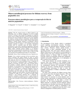
considers all of these areas. We can see in the figure 1.1 the regional differences between
advanced and third-world countries.
Figure 1.1: Ecological debtor and creditors. Source Living Planet Report, 2006. In table 1.1 we can see some ecological footprint indexes: important differences we note
from “northern” and “southern” world countries.
Freshwater is not included in the ecological footprint because it cannot be expressed in
terms of global need hectares that make up this index. It is nonetheless critical to
ecosystems and human population.
8 Introduction
Country
World
United Arab Emirates
U.S.A.
United Kingdom
Greece
Russian Federation
Italy
Brazil
China
Egypt
Morocco
India
Population (millions)
6301.5
3
294
59.5
11
143.2
57.4
178.5
1311.7
71.9
30.6
1065.5
Ecological footprint per capita
2.23
11.9
9.6
5.6
5
4.4
4.2
2.1
1.6
1.4
0.9
0.8
Table 1.1: Ecological footprint (global hectares per person in 2003). Source Living Planet Report, 2006. Freshwater is far from equally distributed around the world, and many countries withdraw
more water than can be sustained without having placing pressure on the land and
ecosystems. A useful indicator is the withdrawals-availability ratio, that measures the
annual water use by the population against the annual renewable water resource. The higher
the ratio, the greater the stress places in freshwater resource. Withdrawals of 5-20%
represent mild stress, 20-40% represent moderate stress, more than 40% severe stress
(Hails, 2006). For instance the U.S.A. freshwater withdrawals, including that for irrigation,
total about 5500 L/person/day. Worldwide, the average withdrawal is 1700 L/person/day
for all purposes (Gleick et al., 2002).
9 Irrigation with saline water: prediction of soil sodication and management
Figure 1.2: Annual water withdrawals per person, by country, 1998‐2002. Source Living Planet Report, 2006. 1.1.1. Water resources and hydrologic cycle
The water present on the Earth is estimated in 1.4 x 1018 m3, and about 97% is in the ocean.
Earth’s freshwater, held in rivers, lakes and reservoirs is about 0.3% (35 x 1015 m3). Some
two thirds of this freshwater is locked up in glaciers and permanent snow cover (UNESCO,
2003). The Earth’s atmosphere contains about 13 x 1012 m3 of water, and it is the source of
rains. The solar energy causes about 577 x 1012 m3 of water evaporation yearly, and the
86% of this becomes from ocean. Thus the 14% of water evaporates from land, but about
the 20% of water precipitations fall on lands (Shiklomanov and Rodda, 2003). This is an
important aspect of the hydrologic cycle that allows the existence of terrestrial’s
ecosystems and human life.
10 Introduction
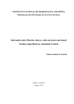
Figure 1.3: Qualitative overview of the hydrologic cycle. However water availability is different among regions, with huge differences in different
parts of the world and wide variations in seasonal and annual precipitation in many places.
The average precipitation for most continents is about 700 mm/y, but this mean varies
among and within them. In fact if we consider the African continent, we observe that has an
average rainfall of 640 mm/y, but there is a great variability between arid and non arid
zones (Pimentel et al., 2004). Regions that receive less 500 mm/year usually have problems
of water shortages and inadequate crop yields. Moreover a nation that has less than
1,000,000 L/head/year is considered with problems of water scarcity (Engelman and Le
Roy, 1993). For example many states of Middle Eastern countries have insufficient
freshwater. The UNESCO 1st World Water Development Report (2003) confirms the
difficulties of many countries around the world (table 1.2). Thus we need to manage water
resources and we need to consider agricultural, environmental and societal systems all
together because they need great quantities of water.
11 Irrigation with saline water: prediction of soil sodication and management
Region
Water availability per capita
(m3/year)
Canada
94353
Congo, Dem. Republic
25183
France
3493
Italy
3325
Morocco
971
Egypt
859
Israel
276
Jordan
179
Saudi Arabia
118
Table 1.2: Quantity of water available per person/year. Source UNESCO 1st World Water Development Report, 2003. 1.1.2. Water use in the world
The increase of population and of its wellbeing gives serious problems at water resources.
Now we use water for all aspects of our life. Even if agriculture worldwide consumes most
of freshwater, also urban agglomerations and industries give several problems to water
resources. Presently 48% of world’s population lives in towns and cities; by 2030 this will
rise to about 60%. Moreover countries that most urbanized in the past forty years are
generally those with the largest economic growth. Urban areas generally provide the
economic resources to install water supply and sanitation, but they also concentrate wastes.
Where good waste management is lacking, urban areas are among the world’s most lifethreatening environments (UNESCO, 2003). Also industry, fundamental part of the global
economy, requires adequate resources of good water. Global annual water use by industry
is expected to rise from an estimated 725 km3 in 1995 to about 1170 km3 by 2025, by
which time industrial water usage will represent 24% of all water abstractions. There are
some differences in water use for different part of the world, in fact it is assumed that
industry is more present in developed countries. Figure 1.4 shows industrial, domestic and
agricultural usage for similar regions of the world (UNESCO, 2003):
12 Introduction
Figure 1.4: Water distribution uses in the world. Source UNESCO, 2003. Problems with water pollution by industry are not restricted only to freshwater, but the
threats are also for coastal zones that are increasing concentration of industry and
population. So that habitats and water of coastal areas are under great stress. In addition air
emissions of persistent organic pollutants, for example, may pollute waters far removed
from industrial centers (UNESCO, 2003).
At last we can say that water needs for human activities is in great increase and the main
problems are pollution and reduction of water resources due to its major request.
1.2.
Agriculture and irrigation water
Humans obtain all their nutrients from crops and livestock and these nutrient resources
require energy, land and water for the productions. The importance of irrigation in
agriculture is underlined when we consider that approximately 17% of croplands worldwide
are irrigated and they produce about 40% of the world’s food (FAO, 2002). Because of the
increasing of world population we need to increase the irrigated areas, and this is possible if
we rise the efficiency of water use. In fact water is already in very short supply in several
countries, and many others also suffer locally from severe shortages (FAO, 2002). When
we deal with water shortages and crop productions it should be useful to consider even that
livestock requires a great quantity of energy and thus water resources, because of the
passage from one step to another in the “trophic pyramid”, where trophic pyramid means
the flux of matter and energy from one organism to another. In fact it is estimated that in
13 Irrigation with saline water: prediction of soil sodication and management
each level passage the energy available reduced on a factor 10. Hence, the loss of energy as
it passes from producers to primary consumers even explains the increasing quantity of
water requested. This aspect involves that the energy requirement for the production of a
certain quantity of meat is comparable as ten times the energy for the production of forages.
Table 1.3 summarizes the request of water to produce 1 kg of forage crops (Pimentel et al.,
1997). The last line of the table refers to the water demand to produce 1 kg of beef meat:
Crop productions
L/kg dry mass
Potatoes
500
Wheat
900
Alfalfa
900
Sorghum
1100
Corn
1400
Rice
1900
Soybeans
2000
Beef
43000
Table 1.3: Request of water for different crop productions. The last line refers to the quantity of water requested to product 1 kg of beef. Source Pimentel et al., 1997. It is important to understand the large quantity of water used in livestock systems because it
allows to evaluate these productions in terms of water needed for the soil. In fact producing
1 kg of beef requires about 43 times more water than producing 1 kg of grain (Pimentel and
Pimentel, 1996). If we consider the quantity of water directly required from livestock we
need only 1.3% of the total use in agriculture. But if water for crop productions requested
by livestock is included, this dramatically increases the water requirement. Producing 1 kg
of fresh beef requires 13 kg of grain (USDA, 2001) and 30 kg of forage (Heischmidt,
1996). So that the sum of water requested for both grain and forage is 43,000 L and it
becomes relevant to find alternatives at good quality water and to increase the efficiency of
irrigation systems. For instance reducing pollution of water used by industries, farms and
urban areas would enable much more of it to be re-used in agriculture. In fact there are
enormous potential benefits from use of wastewater in agriculture. As an example we can
consider that the water of a city that reaches the public sewerage system is more or less
80% of water used. If it is well treated there are many possibilities of using carefully this
water. The fertilizer value of the effluent is almost as important as the water itself. Typical
14 Introduction
concentrations of nutrients in treated wastewater effluent from conventional sewage
treatments are: nitrogen, 50 mg/L; phosphorus, 10 mg/L; and potassium, 30 mg/L (FAO,
2002). If we consider the Italian law limit of 170 kg/ha of nitrogen per hectare, we can use
a quantity of water that is 3400 m3/ha. Considering a city of 500,000 inhabitants that use
generally 120 L per day of water, we obtain totally 48000 m3/day; finally we could irrigate
5000 hectares. In addition we can consider that most of these nutrients should be adsorbed
from crops, with obvious advantages for quality rivers (FAO, 2002). We can conclude that
the correct use of water resources, that means also the possibility to use saline or non
conventional water, such as domestic or zootechnical wastewater, subdued to different
depurative process, should be one of the key to guarantee the water necessity and
maintaining good quality of the soil and ecosystems.
On the other hand agricultural ecosystems, that allow to maintain the food production, need
to be well protected to guarantee crop yields; the closer the agricultural system is to the
natural ecosystem, the more sustainable it is, because less environmental degradation takes
place in the less intensively managed system. This aspect becomes important when we deal
with water management, because water can be best conserved in the fields, as nutrients, by
controlling soil erosion and water runoff and by maintaining a good quantity of organic
matter in the soil. A better water management also means less input of energy. It is
estimated, for example, that United States invest large amounts of fossil energy input in
agricultural productions into supplying irrigation water – more or less 20% (Pimentel and
Dazhong, 1990), but if water is maintained in the soil we need less quantity of it for crop
productions. Moreover if we have the possibility to use poor quality water it gives
important alternatives to the freshwater used. So that it results that a good quality and good
management of the agricultural ecosystems is fundamental to maintain water quantity. Not
only water management is important for maintaining agricultural ecosystems stability. We
may think about the importance of a correct percentage of organic matter in the soil, or the
importance of species diversity that allows the natural equilibrium of all organisms that live
the same field. In other words, to keep in good conditions the ecosystem can give important
results in terms of land need and steady productions. This aspect involves the hope to
guarantee to the future generations the food needs and productivity of agricultural soils
safeguarding the environment.
15 Irrigation with saline water: prediction of soil sodication and management
1.2.1. Consequences of using wastewater in agriculture
The possibility of using poor quality water for irrigation is important and in many countries
it has already done and continues to be an important source (van der Zee and Shaviv, 2002).
Wastewater is charged with elevated concentrations of chemical compounds in ionic forms
and as suspended soil materials, called dissolved organic matter. Irrigation with wastewater
is associated with a concentrating of compounds due to the loss of part of the water from
the soil system by evapotranspiration, whereas chemicals cannot. This aspect is particularly
underlined in arid and semiarid regions, where the ratio of water that evaporates is high.
The difference between soil and water mechanisms is correlated with the different time in
which processes become. In fact changes in the soil, different from atmosphere and water,
occur slower because the buffering mechanisms that oppose changes are much more
profound. It implies that we can obtain good results of maintaining in good conditions the
soil quality, on the other hand a bad wastewater management can have disastrous
consequences with impossibility to remedy in short times. Using wastewater can get
advantages in more water for the crops and also can improve fertilization of soil and crop
at the same time. Moreover we remove pollutants from water that are adsorbed by the soil
and used by plants, and we also create economic value of something that was considered
only a cost (van der Zee and Shaviv, 2002). On the other hand crop requests may be
different from water composition, so that we can find problems of chemicals accumulation.
Soil accumulation of such monovalent ions compromises soil properties due to the
deterioration of its structure. The problem becomes great when we deal with sodicity. In
wastewater, especially if it arises from domestic wastewater, a relatively high Na+ content
may be expected. Sodicity problems arise slowly, but once soil deterioration occurs within
short times and reasonable economic costs sodic soils are rarely remedied. The unbalance
between monovalent and divalent cations causes swelling and shrinking behavior of soils
with a certain quantity of clay. Swelling causes a major non permeable behavior that does
not allow good quality water to enter the soil. It means that the problem of supplies of water
increases. When this problem become evident the necessity of leaching is almost
impossible because of the loss of permeability. Another problem of using this kind of water
deals with heavy metal accumulation, with bad consequences for both crop growth
inhibition and soil pollution (van der Zee and Shaviv, 2002). This can even imply the
possibility to pollute groundwater resources. Nowadays water treatments avoid this
16 Introduction
problem and metal contents are usually reduced to such a degree, so that the problems are
not expected, but it does not mean we need to pay less attention at all water parameters.
1.2.2. Salinity problems in irrigation
The consequences for present and future times of salt accumulation in the soil use are
significant, even more if we consider that often salinity problems can be correlated with
sodicity ones. Consequences of salinization include (Monatanarella, 2006):
ƒ
loss of soil fertility due to toxic effects of high salt contents;
ƒ
reduced water infiltration and retention resulting an increase water run-off;
ƒ
damage to transport infrastructure from shallow saline groundwater;
ƒ
damage to water supply infrastructure;
ƒ
loss of biodiversity;
ƒ
land value depreciation.
Many agricultural practices cause alteration of soil attributes that result in soil malfunction
and degradation, and soil quality is a critical component of sustainable agriculture. The use
of non conventional water resources can give serious consequences to crop productions and
soil if management is not correct. Soil salinity problems and irrigation with saline water are
widespread and it is estimated that include one third of all irrigated lands. Both humid and
arid, semiarid regions are involved in this problem, even if it is more present in the second
one. For example there is salinity soil hazard in Australia, India, Middle East, Southwestern
U.S.A., that are commonly arid and semiarid; nevertheless we have the same problems in
Sweden, Holland and Hungary. Also the Mediterranean basin is interested in this matter
(Yaron, 1981). It has been estimated that 100,000 acres per year of land (nearly 250,000 ha)
are no more productive due to salinity problems (Evans, 1974). This aspect will be
discussed better in the section 1.3.
The salinity problem is more acute in arid and semiarid regions due to the need of extensive
irrigation, low annual rainfall that is not enough to meet evaporative need crops and relative
scarcity of good quality water. Thus, even with relatively good quality water, the permanent
irrigation practice causes the irrigated soil to be affected by an excess of soluble salts
(Bresler, 1982). Moreover, world prospects indicate that the quality of the irrigation water
17 Irrigatiion with salinee water: prediction of soil sodication
s
andd managemennt
tends to deteriorate,
d
so there is the necessity of using
g poor quallity water. IIn this situaation
there is ann accumulaation of salts in the land and the so
oil becomess saline. It iis demonstrrated
that probblems relateed to salt concentratiions are offten presennt in areas with drain
nage
problems (Yaron, 19982). In thiis case watter, that harrdly drains, evapotransspires and salts
s
accumulaate in the fieeld.
1.2.3. Efffect of salinity in crop
p productio
ons
fer from highh salinity leevels of irrig
gation waters because oof high osm
motic
Crops gennerally suffe
pressure that
t
inhibitss water sucction. Cropss symptomss from highh salinity arre generally
y the
same as symptoms
s
o moisture stress from
of
m dry condittions. Dissoolved salts ccause plant cell
dehydration by deccreasing thee osmotic potential of
o soil waater. Figuree 1.5 show
ws a
qualitativve behavior of plants grrowth at diff
fferent soil solution
s
conncentrationss.
Figurre 1.5: Differe
ent water extrraction with low salinity (A
A) and high saalinity (B) in so
oil solution. Table 1.44 summarizees crop foraages and veegetables th
hat suffer frrom salinityy. Salt sensiitive
species produce
p
greeat yield reeductions ovver a very narrow rannge of soill salinities. For
instance bean
b
producction reducees of 10% at
a only 1.5 mS/cm of extracting
e
w
water, whilee 3.5
mS/cm iss enough too reduce off 50% the production.. Others aree more toleerant, as wheat
w
(Triticum eastivum L.)
L and talll fescue (Feestuca arun
ninacea Schhreb.). The examples show
that is posssible and helpful
h
to usse saline waater, but it must
m be pay attention. S
Since salinitty of
the soil will
w not be leess than thatt of the irriggation waterr, the range of irrigatioon water saliinity
that allow
ws maximum
m yield is reestricted forr sensitive crrops.
18 Introduction
Crop
Allium cepa L.
Beta vulgaris L.
Daucus carota L.
Festuca arundinacea Schreb.
Lactuca sativa L.
Lolium perenne L.
Lycopersicon esculentum Mill.
Oryza sativa L.
Phaseolus vulgaris L.
Solanum tuberosum L.
Trifolium pretense L.
Triticum aestivum L.
Zea mais L.
ECe x 103 mS/cm at 25° C at which yields decreased by:
10%
25%
50%
2
3.5
4
10
13
16
1.5
2.5
4
7
10.5
14.5
2
3
5
8
10
13
4
6.5
8
5
6
8
1.5
2
3.5
2.5
4
6
2
2.5
4
7
10
14
5
6
7
Table 1.4: Salt tolerance of plants; ECe refers to electrical conductivity of extracting water. Source Bernstein, 1982. When poor soil conditions prevent adequate leaching or when water management is not
good, much lower irrigation of poor quality can eventually cause salt accumulation in the
soil. Sodicity is another problem connected with salinity. Often the two problems are
linked, in fact usually salinity and sodicity problems are in the same kind of water. Sodic
soils inhibit plant growth because of unfavorable soil conditions and potential deficiencies
of calcium and magnesium (Bernstein, 1982). The first of the two aspects above is
correlated with the loss structure of the soil and it means lack of oxygen because of the
occlusion of pores by the soil particles. All plants reduce their production with loss of soil
structure as a result of high sodium content. On the other hand, even if high salt level can
inhibit crop production, it keeps and improves soil structure by promoting flocculation and
tends to maintain certain levels of calcium and magnesium. The measurable effect is an
adequate keeping of exchangeable divalent cations.
1.2.4.
Salinity water parameters
The most important parameter for saline water and its management is the total
concentration and total quantity of dissolved salts. One of the first used parameter to this
aim is called Total Dissolved Solids (TDS), which considers the total amount of all organic
19 Irrigation with saline water: prediction of soil sodication and management
and inorganic compounds contained in a liquid and that are present in molecular or ionized
form. It is determined by evaporating from a water sample to dryness and weighing the
quantity of salts remaining. The U.S. Salinity Laboratory Staff (1954) collected a
representative sample of surface water and groundwater, and it seems to be a clear method
of water classification. But several remained salts often contain a variable amount of water.
Values were usually reported in ppm (parts per million) TDS, although now sometimes is
preferred milligrams per liter (mg/L). There are no relevant differences between the two
sets of units when we deal with irrigation waters, although numerically mg/L are somewhat
larger than ppm because of different solution densities. In fact salt water is heavier than
pure water. Groundwater and surface water have generally different range of dissolved
solids. The U.S. Salinity Laboratory Staff (1954) reported lowest values for irrigation
waters equal approximately 75-100 mg/L, found in the western U.S.A. The total quantity of
dissolved solids normally increases with increasing distance from the river’s head, as a
result of mineral weathering. Even for high quality river salts concentration are commonly
10-20 times greater than those present in precipitation. More typical levels of dissolved
solids measure approximately 250-900 mg/L. Water with high concentration of dissolved
salts becomes more dangerous for crop productions and fine-textured soils. However,
irrigation waters used in Salt River Valley of central Arizona sometimes approach TDS
values from 2,000 to 3,000 mg/L, and also in Texas has been used water with 4,000 mg/L
of TDS (McNeal, 1982). More saline waters must be used carefully and it should be
guaranteed the correct management. For instance the practice of leaching requirement could
be one of the solution to the problem. Groundwater used for irrigation usually contains
higher TDS levels than to river water of the same region. The lowest reported TDS value
commonly 200-300 mg/L, with well waters levels till 2,000-3,000 mg/L. The higher levels
are due to selective withdrawals of water by plants in the groundwater recharge area and to
dissolution of minerals in the soil and rocks when water flows (McNeal, 1982).
Another method to evaluate the total quantity of dissolved salts is the electrical conductivity
(EC) of the water. This method is now preferred because TDS is more ambiguous and
requires time and technologies that now are out-of-date. The determination of EC involves
placing two electrodes in a sample of water, imposing an electrical potential difference. It is
so measured the resistance of the solution. As the salt concentration increases also the
ability to transmit electricity increases. Results are usually converted from electrical
resistance to electrical conductance and they are usually referred to temperature equals
20 Introduction
25°C. The unit measure is usually mS/cm, which is equal to mmhol/cm, that is referred to
resistance (ohm). The U.S. Salinity Laboratory Staff (1954) gave an approximate relation
between TDS and mho/cm: TDS (mg/L) ≈ 640 x EC (mmho/cm). From this it results that
commonly irrigation waters would occur in the range of 0.15-1.5 mmho/cm (equals 96-960
mg/L). Another important conversion that we can usually use to find the total cation or
anions in water is: cations - or anions - (meq/L) ≈ 10 x EC (mmho/cm). The U.S. Salinity
Laboratory Staff proposed the following water classification (table 1.5) that highlights
whether there is salinization hazard (Bolt and Bruggenwert, 1976):
EC (mS/cm)
< 0.25
Low salinization hazard
Medium salinization hazard
0.25 < X < 0.75
High salinization hazard
0.75 < X < 2.25
> 2.25
Very high salinization hazard
Table 1.5: Classification of irrigation water with respect to salinity. Source USDA Handbook No. 60, 1954. Another important aspect to evaluate the water quality is the osmotic pressure. In fact plants
behavior to salinity is the expression of osmotic properties and it is linked to it. The
osmotic pressure (OP) is produced by the presence of salts; those salts that produce large
numbers of ions and that remain most completely dissociated into individual ionic
components are those that produce the greatest osmotic effects. If we consider that water
usually has a mixed salts solution, even we assume that the differences of OP are less
pronounced than for single salt solution (McNeal, 1982). So that we can consider
sufficiently valid the relationship there is between osmotic pressure and electrical
conductivity: OP (atm) = 0.36 x EC (mS/L). This value is nearly valid to osmotic pressure
expressed in bar (1 atm = 1.013 bar).
1.2.5. Sodicity problems in irrigation
Aside from their influence on the concentration of the soil solution, the addition of salts to
the soil profile may also lead to an alteration of the composition of the exchange complex.
Such an alteration is typically in the direction of an increase of the percentage of
exchangeable sodium ions, because their salts are the most soluble occurring in nature. The
21 Irrigation with saline water: prediction of soil sodication and management
gradual increase in the sodium saturation of the exchange complex is called the process of
sodication or alkalinization. Generally alkalinization means increase of pH, but it can be
used even for sodium accumulation due to the sodium salts effect of rising pH values. The
rate of sodication process depends on the composition and concentration of the water
supplied to the profile, the amount of water added with irrigation per year and the CEC of
the soil. CEC is the cation exchange capacity, that is defined as the total quantity of cations
that may be retained in the surface layer by electrostatic attraction. Usually it is expressed
in mmolc/100g of soil. This property is typical of clay soils, which are composed by a great
number of layers characterized by residual electrical charges. The sodication effect
generally occurs because of the high solubility of sodium salts, and it is more present if
there is an excess of CO32- and HCO3- over Ca2+ and Mg2+ (Bolt and Bruggenwert, 1976).
The most important phenomena that involve sodium in the soil are swelling, dispersion (So
and Aylmore, 1993) and in consequence erosion. In addition sodic soils become less
permeable even at low salt concentration and water availability for plants reduces. Thus this
problem becomes relevant if we consider the soil quality and its potential crop production.
From antiquity farmers know that sodic soils develop a dark brown surface crust of salts
mixed with dispersed organic matter (Szabolcs, 1989). This condition results from an
accumulation of adsorbed sodium on exchange sites of soil mineral layers and organic
matter, which causes the problems that here are above.
1.2.6. Sodicity water parameters
Irrigation water can create sodic soils and various methods have been proposed to classify
them and their capability to produce sodic soils. Considering the simple Na+ concentration
cannot give good results because at low concentrations sodium can represent alone the 90%
of total cations and can imply sodicity (McNeal, 1982). As a result we will measure low
sodium concentrations, even if the sodicity hazard should be high. The U.S. Salinity
Laboratory Staff (1954) proposed SAR (Sodium Adsorption Ratio) as a useful index for
sodium hazard. This parameter is given by the following relation:
(1.1)
⁄
22 Introduction
Where the cations are concentrations expressed in mmol/L. If we consider that the most
common cations in the water are Ca2+, Mg2+, Na+, while K+ is usually relatively small, we
can conclude that salinity and sodium hazard of a given water can be estimated from any
two of the three parameters: EC, Na+, and (Ca2+ + Mg2+) concentration. Instead we cannot
consider pH as a considerable measure of sodic water because, even if soils with high
values of sodium tend to have pH ≥ 8.5, particularly at low salts concentration this is not a
reliable indicator (U.S. Salinity Laboratory Staff, 1954). Here below (table 1.6) it is
schematized the classification of irrigation water with respect to sodicity:
SAR (mmol/L)1/2
Low sodification hazard
<7
Medium sodification hazard
7< X < 13
High sodification hazard
13 < X <20
Very high sodification hazard
> 20
Table 1.6: Classification of irrigation water with respect to sodicity. Source USDA Handbook No. 60, 1954. At last we can consider the Residual Sodium Carbonate (RSC) as another useful parameter
to classify irrigation waters, because it determines the alkalinization hazard (usually linked
with Na+). When all the Ca2+ and Mg2+ added by irrigation precipitate in the soil as
carbonates, the excess of CO32- and HCO3- will be present as dissolved Na+ (and K+). In the
long period all divalent cations exchanged from the soil will precipitate until the almost
totality of the adsorption complex is saturated with Na+ (Bolt and Bruggenwert, 1976).
1.3.
Salt affected soils and classification
Nowadays salt affected soils are naturally present in more than 100 countries of the world
and many of these regions are also affected by irrigation-induced salinization (Rengasamy,
2006). Based on the FAO/UNESCO Soil Map of the world (2003), table 1.7 emphasizes the
regional distribution of salt affected soils. All the areas shown in the table are not
necessarily arable but cover all salt affected soils around the world.
23 Irrigation with saline water: prediction of soil sodication and management
Region
Total area
Saline soils
%
Sodic soils
%
1899.1
38.7
2.0
33.5
1.8
3107.2
195.1
6.3
248.6
8.0
2010.8
2038.6
1801.9
1923.7
6.7
60.5
91.5
4.6
0.3
3.0
5.1
0.2
72.7
50.9
14.1
14.5
3.6
2.5
0.8
0.8
12781.3
397.1
3.1
434.3
3.4
Africa
Asia, Pacific &
Australia
Europe
Latin America
Near East
North America
Total
Table 1.7: Regional distribution of salt affected and sodic soils. Source FAO, 2003. Soil degradation processes occurring in Europe include erosion, loss of organic matter,
landslides, compaction, contamination by pollutants and salinization. Many recent studies
suggest that there has been in the last decades a significant increase in soil degradation
processes and there are evidences that these processes will increase in the next years if no
action is taken (Montanarella, 2006). The salinity accumulation and sodic problems are
relevant in different grounds; however the problem is even more present in predominant
clay texture soils (Bolt and Bruggenwert, 1976).
The classification of salt affected soils, as presented by the USDA salinity laboratory staff
(1954), is widely used. This classification was created principally for purposes of
reclaiming salt affected soils. It is a simple system based on two criteria:
ƒ
salinity of the soil, which is expressed as electrical conductivity;
ƒ
sodium percentage, which is expressed as ESP (Exchangeable Sodium Percentage).
ESP represents the ratio between Na+ adsorbed in the solid phase and the cation exchange
capacity, which is the maximum quantity of exchangeable cations of a soil and it is usually
expressed in mmolc/100g of soil. There is an important relationship that links SAR and
ESP, hence sodium in the soil solution and in the adsorbed phase (U.S. Salinity Laboratory
Staff, 1954):
0.015 (1.2)
Different ranges of ESP were proposed to define sodic soils: for instance the U.S. Salinity
Laboratory Staff (1954) proposed sodic soils with ESP more than 15, while in Australia it
considers ESP ≥ 5. There are also studies that show how even soils with ESP ≤ 1% exhibit
24 Introduction
sodic behavior (Sumner, 1993). In fact this parameter is related with soil properties and the
EC of irrigation water. However usually SAR and ESP are similar, and the higher is SAR
value the more similar is ESP. Finally we can say that the classification of irrigation water
should consider at least EC and SAR to define a good management of all, and especially
non conventional, waters. In fact the problem of sodicity arises when it occurs water with
low EC values, either through good water applications or rainwater falls (Halliwell et al.,
2001):
SAR
0-3
3-6
6-12
12-20
> 20
No problem
> 0.9
>1.3
> 2.0
> 3.1
> 5.6
EC (mS/cm)
Slight to moderate
0.9-0.2
1.3-0.25
2.0-0.35
3.1-0.9
5.6-1.8
Severe problem
< 0.2
< 0.25
< 0.35
< 0.9
< 1.8
Table 1.8: Guidelines for interpretation of water quality for irrigation. Source Halliwell et al., 2001. At low concentration adverse physical effects of a high ESP value will appear early, while
the opposite conditions we have with high salinity of irrigation water.
Due to its simplicity, the USDA classification of salt affected soils does not be applied for
all situations and all soils indiscriminately, because there are variations occurring in nature
that here are not considered, for instance there are not references about the soil texture.
However the major part of soils have characteristics that can allow us to use this
classification with a certain confidence.
1.3.1. Saline soils
Saline soils have a conductivity of the saturation extract more than 4 mS/cm at 25° C and
ESP is less than 15% (U.S. Salinity Laboratory Staff, 1954). When adequate drainage is
established the excessive soluble salts may be removed by leaching and they again become
normal soils. They are recognized by the presence of white crusts of salts on the surface.
The chemical characteristics are mainly determined by the kinds and amounts of salts
present. Owing to the presence of excess salts and the absence of significant amounts of
exchangeable sodium, saline soils generally are flocculated. As a consequence permeability
is equal to, or higher than, that of similar non saline soils.
25 Irrigation with saline water: prediction of soil sodication and management
1.3.2. Saline-alkali soils
Saline-alkali is applied to soils for which the conductivity is more than 4 mS/cm at 25° C
and the exchangeable sodium percentage is greater than 15%. These soils form when
salinization and sodication processes combined together. As long as excess salts are
present, the appearance and properties of these soils are generally similar to those of saline
soils (U.S. Salinity Laboratory Staff, 1954). The pH is seldom higher than 8.5 and the
particles remained flocculated. If the excess soluble salts are leached downward, the
properties may change and become similar to those non saline-alkali soils. As the
concentration of the salts in the soil solution is lowered, some of the exchangeable sodium
hydrolyzed and forms sodium hydroxide. This can change to sodium carbonate upon
reaction with carbon dioxide adsorbed from the atmosphere. In any event, upon leaching,
the soil may become strongly alkaline (pH more than 8.5), the particles disperse and the soil
becomes unfavorable for the entry and movement of water and for tillage. The management
of saline-alkali soils continues to be a problem until the excess of salts and exchangeable
sodium are removed from the root zone and a favorable physical condition of the soil is
reestablished.
1.3.3. Nonsaline-alkali soils
Nonsaline-alkali is applied to soils for which ESP is more than 15% and the electrical
conductivity is less than 4 mS/cm at 25° C (U.S. Salinity Laboratory Staff, 1954). The pH
value is usually more than 8.5, sometimes till 10. These kind of soils usually occur in arid
and semiarid regions. The drainage and leaching of saline-alkali soils usually lead to the
formation of nonsaline-alkali soils. Dispersed and dissolved organic matter present in the
soil solution of highly alkaline soils may be deposited on the soil surface by evaporation,
thus causing darkening and giving rise to the term “black alkali”. The ESP present in
nonsaline-alkali soil may have a marked influence on the physical and chemical properties.
As the proportion of exchangeable sodium increases, the soil tends to become more
dispersed. The pH can also increase as high as 10. At these pH values the composition of
soluble salts in solution may vary a lot from that of normal and saline soils. While the
anions present consist mostly of chloride, sulfate and bicarbonate, small amounts of
carbonate often occur. In fact at high pH calcium and magnesium with carbonate ions are
26 Introduction
precipitated, hence the soil solution of these soils usually contains a few quantities of these
cations and sodium is predominant. Sometimes large quantities of soluble potassium may
occur in these soils.
1.3.4. Salinity and sodicity problems in Europe
The problem of land degradation concerning salinity and alkalinity in Europe limits the
satisfactory utilization of soil in many regions and causes planning problems in both
agricultural and environmental aspects. Frequently soils become salinized and/or
alkalinized because of human activities such as inadequate irrigation management of
agricultural lands. Salinization affects around 3.8 million ha in Europe and most affected
are Campania in Italy, the Ebro valley in Spain and the Great Alföld in Hungary, but also
areas in Greece, Portugal, France, Slovakia and Austria (Monatanarella, 2006). There are
also evidences that the occurrence of salt affected soils in Italy is located along the coasts of
mainland and some regions of Sardinia and Sicily (Szabolcs, 1989). The problem certainly
exists even due to the widely irrigation practices occurring in the territory.
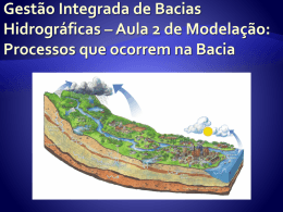
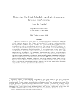
Figure 1.6: Salt affected soils in Europe. Source Szabolcs, 1989. 27 Irrigation with saline water: prediction of soil sodication and management
1.3.5. Salinity problems in Italy Salinity of soils in Italy is not a widespread phenomenon now, but there are some aspects
that may be decisive for the arise of this problem in large scale. At first the overexploitation
of the groundwater may cause the fall of water table level and the consequent intrusion of
seawater, especially along the coasts. This aspect may cause the presence of saline water
and the following withdrawals. Hence the problem arises because that saline water is used
for irrigation and it should be particularly marked in regions with high percentage of
agricultural lands.
Figure 1.7: Intrusion of seawater due to excessive withdrawals. Source APAT, 2007. On the second hand the need of using wastewater is increasing globally, especially in
agriculture, thus the contribution of salts is clearly more than using freshwaters. At last arid
lands will increase due to the effects of climate change (Malhi et al., 2002), hence there will
be less leaching and more evapotranspiration with the consequent arise of new saline soils.
The geographical position of Italy allows to predict the possibility of growing salinity and
sodicity problems. Nowadays there are evidences that the problem is in the low Po valley,
Tyrrhenian and Adriatic coasts and major islands, i.e. Sardinia and Sicily (APAT, 2007).
Seawater intrusion is also one of the main problems of coastal alluvial plains, which are
used intensively for agriculture and industry purposes (Tedeschi and Dell’Aquila, 2005). As
a consequence of the effect of seawater they are all saline soils dominated by effect of
28 Introduction
sodium chloride. Hence the salinity problem becomes more dangerous even due to sodic
accumulation (Szabolcs, 1989).
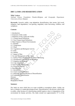
Figure 1.8: Distribution of saline soils. Note that 10% of Sicily lands has problems of salt accumulation. Source APAT, 2007. 1.3.6. The Veneto region situation
In the Veneto Italian region there are problems due to the loss of organic matter, erosion,
pollution and salinization. The presence of salt affected soils in Veneto is caused by
subsidence of brackish and lagoon areas, and even due to the withdrawals of great quantity
of groundwater for industry, civil use and agriculture (APAT, 2007). Studies demonstrated
that the major problem is along the coast, where the seawater intrusion causes salinization
due to the natural and man-induced subsidence (Tedeschi and Dell’Aquila, 2005).
29 Irrigation with saline water: prediction of soil sodication and management
Figure 1.9: Veneto region areas characterized by saline soils or with major salinization hazard. Source APAT, 2007. 30 2. STUDY OF SENSITIVITY OF ESP TO DIFFERENT SOIL CONDITIONS
2.1.
Introduction
Measurements on sodication soil processes usually are not made under the same initial
conditions. Different countries and different studies often have not the same standard state;
for instance it is not used the same solid:solution ratio, or studies have been done at field
capacity, but the soil moisture can change because of different physical soil conditions.
Thus there could be not harmonization on results of experiments and assumptions that have
been made, such as values on the exact adsorption ratio of the major monovalent and
divalent cations that is settled by the exchange equilibrium (in our case, in fact, we will
consider Na+ and Ca2+). The exchange equations are the main point to predict changes in
the soil system as a result of external inputs, such as fertilizers, ion uptake by plants,
irrigation practices and possible wastewater use.
The problem arises when the initial conditions, such as soil moisture, or the addition of
water and cations in the soil, are not the same. There are evidences that experiments are
sometimes made with a certain solid:solution ratio (USDA, 1954; White, 1966; Puls et al.,
1991), or at field capacity and in the saturated paste (Stivens and Khan, 1966; Bolt and
Bruggenwert, 1976; Everest and Seyhan, 2006); these last two are soil characteristics that
can change from one site to another and may have effect in the soil measures that we need
to do. Other times different salt concentrations or CEC are used (McKenzie, 1951; Bayens
and Brandbury, 2004). Hence we need a relationship between the exchange complex and
the soil solution to determine the exact exchange equilibrium between monovalent and
divalent cations that are involved in the adsorption processes. At last we need to assess how
big differences there are between ESP* (a new estimated value of ESP) and the ESP value
that is given as initial parameter, after changing inputs that are CEC, water added in the soil
system (r, ml/100g), the moisture of the soil (w, ml/100g) and the total salt concentration in
the soil solution (Ctot, mmolc/ml). Hence different initial conditions could have different
effects in the exchange complex and soil solution. In our case we have a simplified
situation where, as mentioned before, we consider only the principle monovalent and
divalent cations, i.e. sodium and calcium.
31 Irrigation with saline water: prediction of soil sodication and management
2.2.
The Gapon equation
Before explaining the scheme of calculations and results that have been obtained, it is
fundamental to introduce the Gapon exchange equation. In fact the rate of the different
cations that are in the solid and solution phases is balanced by exchange equations. In our
particular case we will consider an heterovalent exchange, in fact we will assume the
exchange equilibrium between the most common monovalent and divalent cations in a soil
system, i.e. Na+ and Ca2+. Experimental data have shown that for most soils the monodivalent equilibrium is characterized by the following equation:
⁄
(2.1) where KG is the empirically determined Gapon exchange constant and γ+ and γ2+ refer to the
monovalent and divalent cations adsorbed in the solid phase (in our case sodium and
calcium), while Na+ and Ca2+ refer to sodium and calcium in the soil solution phase. The
Gapon constant KG has the [concentration]-1/2 dimension. Hence, if the concentration both
for monovalent and divalent cations is expressed in terms of moles, usually soils exhibit a
1.0
KG = 0.5 (mol/L)-1/2.
Fraction of Ca adsorbed
0.4
0.6
0.8
0.2
Tot_Conc=0.01
Tot_Conc=0.15
Tot_Conc=0.30
Tot_Conc=0.80
Tot_Conc=2.00
0.0
0.0
0.2
0.4
0.6
0.8
1.0
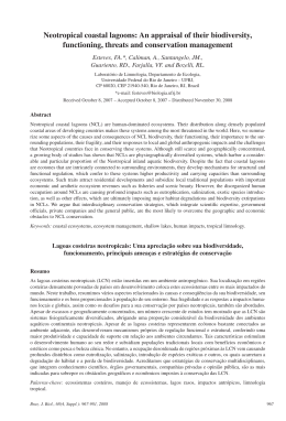
Fraction of Ca in soil solution
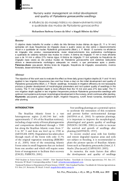
Figure 2.1: Gapon equation with different salt concentrations (molc/L). The figure shows different divalent‐monovalent soil affinity changing the total concentration in soil solution. 32 Study of sensitivity of ESP to different soil conditions
The main limitations are underestimation of the exchangeable Na+-percentage in the high
range (> 40% Na) and in montmorillonitic soils, where KG tends to be close to unity (Bolt
and Bruggenwert, 1976). The Gapon equation is the simplest and reliable mono-divalent
exchange equation which may be used in all those cases where no information is available
as to the particular conditions locally.
2.3.
Calculations of ESP*
The solid phase particles of the soil often carry a negative surface charge. The overall
electroneutrality of the system is maintained by the presence of an excess of cations close to
the solid surface. It is possible to exchange these cations against others, while maintaining
the electroneutrality of the system by means of the replacing cations. The total amount of
the cations exchangeably adsorbed by the complex system is the CEC, which is expressed
in mmolc/100gsoil. All cations are adsorbed in different concentrations by the negative
surface charge and the exchange reactions on surfaces are very high. Once the equilibrium
has been reached there exists a relationship between the composition of the exchange
complex and the soil solution. In soil science history many studies have attempted to
generalize this relationship using exchange equations, but no one has found an exchange
equation valid for all different exchange materials in the soil; however it states that often a
reasonable accuracy is found with equations that only depend on one empirical parameter.
As highlighted in paragraph 2.2 experimental data have shown that for the most soils the
mono-divalent exchange equilibrium follows the Gapon equation, that here we will write in
terms of fraction of sodium (fNa) and Ctot (mmolc/ml), i.e. total salt concentration:
(2.2)
where γ+ and γ2+ refer respectively to the quantity of monovalent and divalent cations in the
adsorbed phase (expressed in mmolc/100g soil) and the Gapon empirical constant is
expressed in (mmol/ml)-1/2. Changes occurring in the field that influence the exchange
equilibrium may be summarized as additions (positive and negative) of ions and/or water.
In our special case we consider only the addition of water. Hence the Gapon equation can
be written as (Bolt and Bruggenwert, 1976):
33 Irrigation with saline water: prediction of soil sodication and management
(2.3)
where w is the moisture content of the soil (ml/100g soil), thus wCtot equals the amount of
cations present in the solution of a certain quantity of soil (mmolc/100g). Inputs generate
inequality from left and right hand side of the expression. In this case the input is the
addition of water (r, ml/100g soil) in the soil system, thus we have:
/
(2.4)
where x (mmolc/100g) is the shift of monovalent and divalent cations between solid and
solution phase. We can use x both for monovalent and divalent cations due to the same unit
measure (mmolc/100g) that we consider. Using milligrams or moles instead of millimoles
charge would involve changes in the main equation.
The above equation (2.4) is valid for all cases in which we have addition or extraction of
water; hence the exchange equilibrium, which is present between the solid phase and soil
solution, is reversible and the equilibrium in the soil system can be reestablished as before
the alteration. In this particular case it may be used to calculate the new exchange
equilibrium after irrigation or plant uptake, even if our purpose is to evaluate the variations
in the sodium and calcium fractions in solid and solution phases. The shift of x is settled by
physical conditions (Bolt and Bruggenwert, 1976):
w Ctot fNa x ‐ w Ctot 1‐fNa
(2.5)
The physical meaning of this range is simple: in fact x cannot be more than the real quantity
of monovalent cations that are present in solution, whereas it must be even more than the
initial quantity of divalent cations present in the soil solution. In this special case we
assume that the soil system is characterized by a shift of x (mmolc/100g soil) of monovalent
cations from solution to complex, accompanied by a reverse shift of x (mmolc/100g) of
divalent ions from complex to solution. The opposite argument is for the second range, in
which we have the same shift of monovalent and divalent ions, but in the reverse way:
γ2 x γ
(2.6)
34 Study of sensitivity of ESP to different soil conditions
As said before, in our case we assume only an addition of water (r), which means that x is
always negative, due to the dilution phenomenon; in consequence divalent ions move
towards the complex. If we assume now a soil with a certain high CEC value, and
considering only the movement of divalent cations, we have also that the distribution ratio
(RD = γ+,k/C+,k) is large, where C+,k is a generic concentration of a general cation in solution
and γ+,k is a generic cation in the soil adsorbed phase. It means that the maximum relative
change, i.e. 1/RD, is limited because x must be inside the physical range of equation (2.5).
Moreover the net movement of divalent cations is towards the complex, but there is a low
amount of them respect to the quantity in the complex. The conclusion is that the
exchangeable ratio (left hand side of the equation) is maintained constant. The same
argument, but in the opposite way, is for sodium.
Values of fNa of the main expression (2.4) are obtained from the ESP value, given as initial
parameter, assuming a reasonably ESP range 1-30% (Bolt and Bruggenwert, 1976;
Halliwell et al., 2001). Thus we have:
100 (2.7)
And assuming that (γ+ + γ2+) = CEC we have:
(2.8)
Finally fNa is found from:
0
(2.9)
We assume two possible initial moisture contents (w) equals 1 ml/100g (i.e. considering dry
soil) and 25 ml/100g. In this case we referred to Bolt and Bruggenwert (1976), in which 25
is a reasonable value of soil moisture at field capacity. Generally we keep it constant
(equals 25) to compare different results and due to the fact that for low w values differences
are less evident. Hence we prefer to consider the bigger one to stress how the ESP*/ESP
ratio changes.
Solving equation number (2.4) with respect to x seems to be difficult, in fact it is a 4th order
polynomial equation. However with a different approach, that consists of comparing the
right hand side with the left hand side (for instance plotting graphically the two different
35 Irrigation with saline water: prediction of soil sodication and management
parts of the equation together), it is easier to obtain the same results of x (Bolt and
Bruggenwert, 1976). Finally the new estimated ESP* is found with the following equation:
100
(2.10)
Table 2.1 summarizes the data set used for the simulations.
Simulations
Line
r
(ml/100g)
w
(ml/100g)
CEC
(mmolc/100g)
Ctot
(mmolc/ml)
ESP
(%)
ESP*/ESP after
changing r, water
added in the soil
I
II
III
50
100
200
25
25
25
30
30
30
0.01
0.01
0.01
1-31
1-31
1-31
ESP*/ESP after
changing the
initial salt
concentration
I
II
50
50
25
25
1-100
1-100
0.01
0.002
5
5
ESP*/ESP after
changing the soil
moisture w
I
II
50
50
1
25
1-100
1-100
0.01
0.01
5
5
ESP*/ESP after
changing the
initial given ESP
I
II
2-500
2-500
25
25
30
30
0.01
0.01
15
5
Table 2.1: Initial values used for the simulations to find ESP* value, i.e. the new estimated ESP index. 2.4.
Results and discussion: the ESP*/ESP ratio
Figure 2.2 shows the evolution of ESP*/ESP ratio with respect to the initial ESP value in
three different dilution conditions, which corresponds to an addition of water equals 50
ml/100g, 100 ml/100g and 200 ml/100g. In this case we keep as constant w = 25 ml/100g,
Ctot = 0.01 mmolc/ml and CEC = 30 mmolc/100g. What we can see is that the bigger is r the
smaller is ESP* with respect to the initial ESP, due to the more evident effect of dilution.
With respect to this we consider that we have an extreme situation that arises with
excessive input of the r parameter, corresponding to a large amount of irrigation water.
Now the solution phase is dominant and the soil system will adjust to the composition of
the leaching solution (Bolt and Bruggenwert, 1976). We can also see that for high ESP
values the differences are decreasing till to have no effect of water dilution. This second
aspect refers to the low Ca2+ concentration that is present in the soil-solution system; it
means that there is low flux of divalent cations towards the complex, hence the differences
36 Study of sensitivity of ESP to different soil conditions
we note are very small. This consideration is valid for all samples in which there is a
0.90
0.80
0.85
ESP*/ESP
0.95
1.00
comparison between different initial ESP values.
0
5
r=50ml/100g soil
r=100ml/100g soil
r=200ml/100g soil
10
15
20
25
30
ESP
Figure 2.2: Relationship between ESP*/ESP and initial ESP for different r and keeping constant Ctot = 0.01mmolc/ml, CEC = 30mmolc/100g and w = 25 ml/100g. The figures below (figures 2.3 and 2.4) demonstrate the same trend, however something
changes. In both cases we can see how the ESP*/ESP ratio changes with the CEC range,
but for two different conditions. We consider reasonable values of CEC in the range of
1:100 (mmolc/100g) as expressed in McKenzie (1951), Bolt and Bruggenwert (1976),
Bayens and Brandbury (2004).
In the first case (figure 2.3) we assume two different initial concentrations. The graphic
shows that differences between ESP and ESP* values are bigger when Ctot is high. In this
case w does not change and equals 25 ml/100g. Hence, the bigger is Ctot the smaller is the
distribution ratio for each ion RD = γ+,k/(wC+,k) and so the maximum relative change for
divalent cations (equals 1/RD) towards the complex becomes bigger than for low Ctot values
(here equals 0.002 mmolc/ml). On the other hand, if this effect is clear for low CEC values,
it becomes less evident when CEC is increasing. In fact the system goes to a complex37 Irrigation with saline water: prediction of soil sodication and management
dominated exchange adjustment (Bolt and Bruggenwert, 1976), in which the maximum
relative change is limited. Hence there are less differences between the two situations
expressed above.
In figure 2.4 there are the same initial conditions of figure 2.3 (initial ESP = 5 and r = 50
ml/100g), but in this case w changes and Ctot = 0.01 mmolc/ml. In this case the trend seems
to be the same, even if we have some differences at low CEC values. In fact here the
ESP*/ESP ratio has more differences considering low w, while for increasing CEC we have
the same conditions of figure 2.3. We would expect, as in figure 2.3, that due to the bigger
value of 1/RD, for high w, the maximum change of divalent cations should also be large.
However this is not true when we have low CEC values. Here the comparison between the
0.8
0.6
0.7
ESP*/ESP
0.9
1.0
two lines gives opposite results, so it should mean that the main process is opposite.
0
20
Ctot=0.01 mmolc/ml
Ctot=0.002mmolc/ml
40
60
80
100
CEC (mmolc/100g soil)
Figure 2.3: Relationship between ESP*/ESP and CEC for different Ctot and keeping constant r = 50ml/100g, CEC = 30mmolc/100g and w = 25ml/100g. 38 0.7
0.4
0.5
0.6
ESP*/ESP
0.8
0.9
1.0
Study of sensitivity of ESP to different soil conditions
0
20
w=1 ml/100g
w=25 ml/100g
40
60
80
100
CEC (mmolc/100g soil)
Figure 2.4: Relationship between ESP*/ESP and CEC for different w and keeping constant r = 50ml/100g, CEC = 30mmolc/100g and Ctot = 0.01 mmolc/ml. At last we consider figure 2.5, in which ESP*/ESP is shown in a range of r; ranges of r are
different in different experiments and countries (USDA, 1954; White, 1966; Puls et al.,
1991), but a mean range we consider from 2 to 500 (ml/100g). We assume Ctot = 0.01
mmolc/ml, w = 25 ml/100g and CEC = 30 mmolc/100g. We chose this CEC value because
it is in the range of typical agricultural soils. In fact, as mentioned in Bolt and Bruggenwert
(1976), heavy clay soils exhibit CEC values of up to 40 mmolc/100g.
We can note that for increasing r values the differences in the exchangeable sodium
percentage ratios are more evident, though small and with a minimum of 0.93 for initial
ESP = 5%. On the contrary, with ESP = 15% the ratio is never smaller than 99.3. This
extreme situation arises with excessive input of a parameter. In our case we assume an
increase quantity of water added to the soil system, and, as in figure 2.2, we can assume it
as a particular case in which we have a big quantity of irrigation water. Hence the solution
phase is dominant and the soil system will develop to the composition of the leaching
solution.
39 0.96
0.92
0.94
ESP*/ESP
0.98
1.00
Irrigation with saline water: prediction of soil sodication and management
0
100
ESP initial equals 15
ESP initial equals 5
200
300
400
500
r (ml/100g soil)
Figure 2.5: Relationship between ESP*/ESP and r for different initial ESP keeping constant w = 20ml/100g, CEC = 30mmolc/100g and Ctot = 0.01 mmolc/ml. 2.5.
Conclusions
It is important to determine the exact ESP, from which we can obtain the fraction of sodium
and calcium, because it allows to use reliable data. In fact, as said before, in different
studies usually are used different parameters. Hence it is decisive to understand whether we
can use them directly or where we need to obtain new data. The work here present gives us
important results over this theme. Generally we can say that differences are low and this is
due to the fact that we consider only dilution, thus the range of shifting of ions keeps low.
The introduction of monovalent and divalent cations would give more differences in terms
of shifting of them from the complex to the soil solution and vice versa. It also means that x
is always negative, and it implies that the fraction of sodium in the exchangeable complex
decreases, while calcium is increasing. The main differences we have if we consider low
initial ESP or low CEC. On the contrary, in figure 2.3 and 2.4, if we consider a general
CEC value of 30 mmolc/100g, we note that ESP* has differences almost negligible.
40 Study of sensitivity of ESP to different soil conditions
Figure
2
2-3
3
4
4
r
(ml/100g)
50
50
50
100
300
W
(ml/100g)
25
25
1
25
25
Ctot
(mmolc/ml)
0.01
0.002
0.01
0.01
0.01
CEC
(mmolc/100g)
30
30
30
30
30
ESP
ESP*
5
5
5
5
5
4.853
4.980
4.985
4.791
4.699
Table 2.2: Comparison between different conditions keeping constant certain parameters. Small differences we note also in figure 2.5 (see table 2.2), but here the high r value
influences more ESP* than in the first three cases. Actually these two last conditions
consider amounts of water added of 100% and 300% in weight respect to the soil. It means
that are out of real conditions. However they can suggest how the soil behaves and how big
differences there are for different case studies. At last we can suggest that under extreme
conditions it should be important to check how big are the differences. Using very high
quantity of water or very high saline waters generally implies differences that should be
decisive to understand the problem. Usually it is under these extreme conditions that we
have more evidences about what we are studying. On the other hand, under real conditions,
differences in ESP*/ESP ratio are very small and we can assume that ESP parameter is in
steady state conditions. We can also conclude that sodium and calcium fractions does not
suffer big consequences by different initial conditions. At last we can say that differences in
ESP values under different conditions are usually negligible. The study suggests that the
values of ESP we find in literature are quite harmonized even if the initial conditions are
not the same. Hence the comparison among different sodic soils usually can be done
without allowing for the initial parameters.
41 3. SOIL SODICATION AS A RESULT OF PERIODICAL SALINITY
As mentioned in chapter 1, soil sodication significantly threatens agriculture in arid and
semiarid regions in the world. Sodicity limits the production potential of soils due to affect
on soil structure (So and Aylmore, 1993), such as swelling, dispersion and decrease of
permeability that also involves the loss of water infiltration. As a result plant water uptake
is more difficult and all these aspects mentioned before imply the soil degradation. Sodium
is generally recognized to play a key role in sodication due to the possible high presence of
it in water accompanied by a medium or low level of electrical conductivity, as shown in
table 1.8 (Halliwell et al., 2001). The decrease of water resources and quality will be one of
the most problems in the future (UNESCO, 2003) and to use poor quality water, such as in
irrigation, may give problems of salinization and even more of sodication. Seasonal salinity
already occurs in many arid and semiarid regions because of accumulation of salts in the
root zone unless extra water is added to the soil to leach down the salts. Studies
demonstrate that the problem can arise also in non arid regions (Armstrong et al., 1996;
Tedeschi and Dell’Aquila, 2005). Usually this is mended by leaching requirement during or
after the growing period, but much attention is paid as how to leach the salts (Howell,
1988); on the contrary little attention is paid to possible connection of such a practice to
sodication of soils.
3.1.
Materials and methods
The analytical model that we propose has the aim to describe the behavior both for sodicity
and salinity in a homogeneous root zone, as a result of periodical irrigation with saline
water. The main purpose of the analytical model is to determine and explain the
relationship between salinity and sodicity and to pinpoint the origin of this relation. Hence
keeping in view such a relation we want to describe how the soil sodication process deals
with the soil structure. Using poor quality water we can increase the problem of salinity and
sodicity even where rainfall is quite enough, thus problems may occur also in non arid
regions. In fact the soluble salts that occur in soils consist mostly of various proportions of
the cations sodium, calcium and magnesium, while the anions are usually chloride and
sulfate. Potassium ordinarily occur in minor amounts, as nitrate and carbonate (USDA,
43 Irrigatiion with salinee water: prediction of soil sodication
s
andd managemennt
1954). Heence we asssume a sim
mplified situuation in wh
hich salinityy is due to tthe presencce of
sodium (aalso represeenting potasssium) and calcium
c
(alsso representting magnesium). Chan
nges
in salt conncentrationn and distribbution of caalcium and sodium
s
are calculated as the resu
ult of
infiltration, drainagee and evapootranspiratioon. Thus we
w have fouur sections tthat schemaatize
gure 3.1.
the analyttical model and that aree representeed in the fig
Figu
ure 3.1: Visuall representatiion of the mo
odel in which ssalt concentraation C, calciu
um fraction in soil solutiion (f) and callcium fraction
n in the exchaange complex (N) change in
n time a
as the result o
of infiltration, evapotranspiration and drainage. During onne season the differentt componennts of figuree 3.1 will reach
r
an equuilibrium given
by the initial conditioons we assuume:
44 Soil sodication as a result of periodical salinity
1. infiltration: infiltration water enters the root zone at rate j (L/m2/y) with a certain
salt concentration Cin (molc/L). Infiltration water contains finCin molc/L of Ca2+ and
(1-fin)Cin molc/L of Na+, where f represents the fraction of calcium in solution and
(1-f) the fraction of sodium. Part of the water will evapotranspires at rate τj, where τ
represents the fraction of infiltrating water that evaporates from the root zone. We
reasonably assume that neither sodium nor calcium leave the soil with water that
evaporates. Because the analytical model considers a constant volume of soil
moisture V (L/m2), water drains from the root zone at rate (1-τ)j;
2. soil solution: salts in soil solution we consider VC, where C represents the totals salt
concentration in the soil solution, thus calcium in soil solution is VfC and sodium
V(1-f)C. The salt concentration and composition in the drainage water are assumed
to be identical to those in the soil-solution system;
3. exchange complex: in the exchange complex calcium equals MNγ, where M is the
dry mass of the soil (kgsoil/m2), N is the fraction of calcium in the complex, (1-N)
represents the Na+ fraction and γ (molc/kgsoil) the soil exchange capacity. Infiltration
causes the change of the salt concentration C, and as a consequence it changes even
fC and (1-f)C, calcium and sodium respectively in the solution. Because of the
cation exchange the equilibrium immediately changes, hence Nγ and (1-N)γ change;
4. drainage: water drains at rate (1-τ)j. There is no difference between infiltration from
the top or from the bottom of the root zone, in the form of poor quality water or
capillary rise. In order to calculate the effect of evaporation we select τ = 1, so that
all the water entering the root zone will evaporate.
Thus the model develops in two different conditions: in the first half year we assume
accumulation of salts. In this condition we assume no drainage and τ = 1. On the contrary,
in a second time we have leaching without evaporation, hence τ = 0. Moreover the model
was implemented considering the balance of total salts in the root zone, followed by the
calcium balance.
3.1.1. Salt balance
As suggested above, the first part of the analytical model is the salt balance. Hence we
assume that the change of total salt contents in the root zone (calcium and sodium) VΔC
45 Irrigation with saline water: prediction of soil sodication and management
equals the mass of salt entering the soil jCinΔt and the mass of salt leaving the soil system
(1-τ)jCΔt. We can write this balance in terms of differential equation dC/dt:
(3.1)
The two different conditions we assume are accumulation period and leaching period. The
first one we assume with τ = 1, hence the differential equation will become:
(3.2)
Integration with respect to time means:
And finally the analytical solution is:
(3.3)
In leaching period we will have a different condition, i.e. τ = 0:
(3.4)
We can solve it analytically with the method of variations of constants. Thus the equation
can be rewritten as:
Where (3.5)
and At first we take the homogeneous part and we solve the differential equation:
exp
(3.6) Where U is a constant. We make a trial solution and we assume that U is a function of time.
Again we can find derivation with respect to U (this is because we have the nonhomogeneous differential equation):
’
46 (3.7) Soil sodication as a result of periodical salinity
At last we consider the non-homogeneous part, in which we can combine equation (3.5)
with equation (3.7):
’
Combining again with equation (3.6) gives the following result:
’
’
(3.8)
Now we can integrate to find the value of U:
exp exp
(3.9)
Where k is a constant. Finally, combining equation (3.6) and (3.9) we obtain:
exp
At time t = 0 we find that
exp (3.10)
; hence the final analytical solution for the salt
balance during leaching period is:
exp (3.11)
As expressed above we assume two different conditions that give together one complete
cycle. The values in this calculation have been chosen such that soil salinity at the end of
the year is the same as that of the beginning of that year. Hence the soil is well managed
with respect to soil salinity.
3.1.2. Calcium balance
The second part of the analytical model is the calcium balance. The total calcium content in
the soil system is:
T fCV NMγ
(3.12)
47 Irrigation with saline water: prediction of soil sodication and management
As for the salt balance, also here the change of calcium content ΔT is the difference
between the mass of calcium entering the root zone (jfinCinΔt) and the calcium leaving the
soil system j(1- τ)fCΔt. In terms of differential equation we have:
1
(3.13)
We can rewrite dN/dt in terms of df/dt and dC/dt. In fact N is the fraction of calcium in the
exchange complex, and using an exchange equation it is expressed in terms of calcium in
the soil solution. To do this we use the Gapon equation in which the Gapon constant KG =
0.5 (mol/L)-1/2 (Bolt and Bruggenwert, 1976). This equation shows a bigger affinity for
divalent cations instead of monovalent ones, but this affinity decreases as soon as the
fraction of monovalent ions becomes greater. The Gapon equation (2.1) in terms of N, f
and C reads:
(3.14)
⁄
Hence we can explicit N:
√
(3.15)
If we differentiate with respect to time t we obtain:
√
(3.16)
√
Now we can combine equation number (3.13) with (3.16) which give:
⁄ (3.17)
Equation 3.17 shows how the calcium fraction in solution changes with respect to time. We
can find it numerically, while the evolution of the Gapon equation can be used to find N
simultaneously (equation 3.16). At last total calcium, expressed in figure 3.1 as molc/kgsoil
is obtained from equation (3.13) dividing all by M, dry mass of the soil (kgsoil/m2).
48 Soil sodication as a result of periodical salinity
The integrations of equations (3.1) and (3.17), from which we obtain the salt and calcium
balance respectively, has been made with the classical Runge-Kutta 4th order method using
the R environment and particularly the “odesolve” package (Press et al., 1992).
Combining following seasons gives the possibility to calculate salinization and sodication
hazard and behavior during several years as shown in the next paragraph. Table 3.1
summarizes the data set used for all simulations.
49 50 Initial
parameters
from which
are obtained
64 different
combinations
50-90 years
simulation,
with different
CEC values
90
1 year
simulation.
Accumulation
and leaching
are evaluated
with different
time
0.45
90
0.10
0.03
0.25
0.25
γ
(molc/kg)
0.15
390
390
390
390
M
(kg/m2)
30
90
90
V
(l/m2)
1 year
simulation
Simulations
0.0098
0.0098
0.0098
0.0098
C
(molc/kg)
0.98
0.98
0.98
0.98
f
Initial values
Table 3.1: Data set for different simulations of the analytical model. 900
300
300
300
300
j
(l/m2/y)
0.02
0.02
0.02
0.02
Cin
(molc/kg)
0.60
0.20
0.05
0.05
0.05
fin
0.5
0.5
1
1
900
300
300
0.002
0.002
1
0.33
0.25
0.25
0.25
fin
0.5
t
(y)
0.5
0.5
0.25
0.002
0.002
Cin
(molc/kg)
0.75
300
300
j
(l/m2/y
0.75
1
1
τ
Leaching period
0.25
0.5
t
(y)
Accumulation period
0
0
0
0
τ
Irrigation with saline water: prediction of soil sodication and management
Soil sodication as a result of periodical salinity
3.2.
Results and discussion
Figure 5.2 shows the evolution of total salts, calcium and sodium as the result of periodical
irrigation with poor quality water (Cin,a = 20 mmolc/L, SAR = 19 (mmol/L)1/2) followed by
a leaching period. Referring to the tables number 1.5 and 1.6 we can classify this water as
dangerous for the soil and main crops, due to its high salinization and sodication hazard
respectively. Hence one year is divided into two periods, each one of six months. In the
leaching period water quality is characterized by low electrical conductivity (ECw = 0.2
mS/cm) and lower SAR (equals 2.1 (mmol/L)1/2) than in the first part of the year. We
assume these values reasonably true and they can be compared with tables 1.5 and 1.6
(USDA, 1954). As shown in the figure number 3.2, the salt concentration increases during
the accumulation period because saline water enters the root zone. Moreover we assume
there is not leaching, while all water incoming in the soil evapotranspires (τ = 1). If we
consider that water which leaves the root zone is pure, due to evaporation and plant uptake,
we can easily understand that there is a net salt accumulation in the soil system. After half a
year the accumulation period finishes and the leaching period begins. As a result, the salt
concentration rapidly decreases till initial values. This is due to the assumptions we made,
i.e. values have been chosen such that soil salinity at the end of an entire cycle (one year) is
the same of that at the beginning of the same year. It means we have a good management of
the field with respect to salinity.
Even though the salt concentration in the root zone has not increased at the end of the year,
this is different for the ESP of the soil. As we find in literature (Bolt and Bruggenwert,
1976; Halliwell et al., 2001) sodication hazard arises when, after a period of irrigation with
high saline water, there is a following period characterized by water with low EC, such as
rainfall. As a consequence swelling and dispersion will be the main problems of the soil
system, though are buffered when wastewater remains in the soil over certain critical
flocculation values. This is the situation in which we presumably are, even though here we
focus in the sodication process and not in its consequences. The results of figure 3.2
demonstrates that sodium content both in soil solution as well as in the exchange complex
increase, due to the high sodium fraction of irrigation water (1-f = 0.95). Also ESP
increases: if at the beginning we have ESP = 0.14%, due to extreme initial conditions we
assume, at the end of accumulation period ESP = 2.4 (with CEC = 25 mmolc/100g). As a
result of high salt concentration and high SAR, sodium added with irrigation water is
51 Irrigation with saline water: prediction of soil sodication and management
exchanged with calcium content of the exchange complex. This is due to the decreasing
affinity of the complex for divalent calcium with respect to monovalent sodium (Bolt and
Bruggenwert, 1976; Appelo and Postma, 2005). In fact the higher charged ions are
preferred more strongly when the total solute concentration decreases. This effect is a
consequence of the exponent that is used in the mass action equation. The graph even
shows how, at the leaching period starts, high concentrated soil solution is leached, whereas
sodium remains almost constant. It means that the major part desorbed is represented by
calcium. The lack of balance between monovalent and divalent cations content in the soil is
even more clear when we focus in the calcium behavior: during accumulation period the
total calcium content is almost constant, due to a limited amount that is present in the
irrigation water that enters the soil system. However we can see that a large quantity of the
divalent cation desorbes as a result of the decrease preference of the exchange complex for
calcium, due to the increase of total salt concentrations. Figure 3.2 even shows that, as soon
as leaching period starts, highly concentrated water rich of calcium leaves the root zone in
order to guarantee leaching in the second part of the year. In fact good quality water is used
for leaching purposes, characterized by low salinity and sodicity levels. At last water
content in the soil solution that leaves the root zone has a quantity of calcium far more
pronounced than the total calcium content. We can conclude that ESP has increased in the
soil due to two main processes: first for the great input of sodium during accumulation
period, and second for the net output of calcium during leaching. It appears that calcium
changes from immobile to mobile phase during accumulation, while it is leached in the
second period because of the addition of good quality water.
52 Soil sodicatioon as a result of periodical salinity
odium and calcium contentts during an accumulation Figurre 3.2: Evolutiion of salt, so
perio
od followed byy a leaching p
period, both o
of half a year. 53
0.253
0.252
0.004
0.251
0.250
0.002
0.249
0.248
0.247
total Na (molc/kg soil)
0.008
0.006
total Ca (molc/kg soil)
Irrigation with saline water: prediction of soil sodication and management
0.000
0.246
0.245
0.0
0.2
0.4
0.6
0.8
1.0
Time (year)
Figure 3.3: 3D representation of both cations (Ca2+ and Na+ in mmolc/kgsoil) in the soil system with respect to time, during accumulation and leaching. This is also proved when the calcium behavior has been compared in the three different
scenarios below, in which the time of accumulation and leaching changes (figure 3.4). As
explained before it states that the calcium content in the soil has been changed to the soil
solution during the accumulation period.
54 Soil sodicatioon as a result of periodical salinity
Figu
ure 3.4: Total ccalcium (solid
d lines) and exxchange comp
plex (blue dottted lines) behavior with th
he changing tim
me of accumu
ulation and leaching. Initial data have be
een assumed the same of tthe figures 3.2 and 3.3. Thee figure bellow (3.5) exxplains bettter the behaavior of callcium between soil sollution and
exchange com
mplex. In faact the majoor part of calcium in desorbed dduring accu
umulation,
wheereas the frraction in soil solutionn seems nott to have a great increease, due to
o the high
quaantity of saltts that is alrready preseent in the water. On thee contrary in leaching period the
fracction of calccium in the exchange complex
c
is almost
a
at stteady state, while theree is a great
decrease in soiil solution, due
d to the leaching
l
efffect. Eventuually sodium
m has a greaat increase
in the
t exchangge complexx during acccumulation period, whhile it keepps almost constant in
leacching. This is in agreem
ment with thhe opposite calcium behhavior.
55
1.000
Irrigation with saline water: prediction of soil sodication and management
0.990
0.975
0.980
0.985
t=0.25
t=1
t=0.75
t=0.5
0.965
0.970
Calcium fraction in adsorbed phase (N)
0.995
t=0
0.7
0.8
0.9
1.0
Calcium fraction in soil solution (f)
Figure 3.5: Relationship between calcium in adsorbed (N) and soil solution phase (f) during accumulation and leaching period. Figure 3.7 shows two similar conditions that differ only CEC. In fact we can see the
behavior of the soil system after several years. In accordance with the model we have, it is
clear that salt concentration does not increase from one year to another, but there is an
alternation between accumulation and leaching, as we expect. The parameters are identical
to those of the figures 3.2-3.6, however we assume CEC of two different soil texture
conditions, especially a low value (CEC = 3 mmolc/100gsoil) and a higher one (CEC = 10
mmolc/100gsoil). CEC has been chosen relatively small to obtain steady state for ESP within
a short period of time, in fact assuming the same CEC of the figures above (CEC = 25
mmolc/100g) the soil system does not reach steady state in a period of 90 years (figure 3.6).
56 25
Soil sodication as a result of periodical salinity
15
0
5
10
ESP (%)
20
CEC = 25mmolc/100g
0
20
40
60
80
Time (year)
Figure 3.6: Sodium accumulation in the soil system for a 90 year time prediction. Both cases (figure 3.7) eventually show a situation in which ESP, that is referred to two
different CEC values, does not change from one year to another, while within the same year
there is a variation due to the accumulation followed by the leaching period. We obtain
these results assuming that the last values of each period must be the first of the next one.
Hence in each period we have initial values, in terms of salt concentration and calcium
fraction, that are the same of the last values of the period before. In this case, as in the
calculations of the figures above (except for figure number 3.4), we consider that each
period is of half a year, thus alternatively we have accumulation and leaching. The same
management of the field is repeated for 50 years. The exchange complex in the soil steadily
equilibrates to the saline and sodic solution which enters the soil in the accumulation
period. In fact it states that in steady state there is a reduction of calcium desorption and
sodium adsorption in the accumulation period as compared to the first few years. Hence
there is less calcium leaching, but more sodium that is leached from the root zone in the
drainage period. At last the soil system reaches steady state when the increase of calcium
57 Irrigation with saline water: prediction of soil sodication and management
and sodium content in the accumulation is balanced by the same monovalent and divalent
Csalt(m
o
lc/l)
0
.0
4
0
.0
3
0
.0
2
0
.0
5
cations content during the leaching time.
0
.0
0
0
.0
1
0
10
20
30
40
50
40
Time (year)
30
Low CEC
20
ESP (%)
High CEC
10
0
0
10
20
30
40
50
Time (year)
Figure 3.7: Salinization and sodication of two different root zone systems that differ only for CEC. Low CEC = 3 mmolc/100g and high CEC = 10 mmolc/100g. 58 Soil sodication as a result of periodical salinity
There are others three aspects that need to be underlined:
1. variations within one year are more buffered with the higher CEC input. This
may be explained if we consider that high CEC values means less percentage
variations of ESP, assuming the same initial conditions;
2. as a result of the former, ESP takes a longer period of time to reach steady state
with high CEC than with low CEC values;
3. it proves that CEC has not real effect on the final ESP as soon as the soil system
has reached the steady state with respect to sodicity. As a consequence different
soil textures could have the same problem on sodication due to this last aspect.
At last figure 3.7 even shows that a higher CEC value buffers the rate of sodication within
one year, whereas it does not play a key role for the final ESP value after the soil system
reaches a certain stability in terms of sodium accumulation. It seems that ESP is given by a
concentrating process in the soil solution because of the negligible effect of CEC. Again, in
figure 3.8 we can see the evolution of the sodium fraction in the soil solution (1-f) in a 3D
representation, with the corresponding fraction in soil solution (1-f), whereas the time is 50
30
0.8
0.6
20
Time (year)
1.0
Na fraction in solution (1-f)
40
50
years, as in the figure above (3.7).
10
0.4
0
0.2
0.00
0.0
0.05
0.10
0.15
0.20
0.25
0.30
0.35
Na in exchange complex (1-N)
Figure 3.8: 3D graphic representation. The fraction of sodium in the exchange complex is related with its fraction in soil solution. CEC = 3 mmolc/100g. 59 Irrigation with saline water: prediction of soil sodication and management
Figure 3.9 demonstrates the evolution of calcium fraction in accumulation and leaching
period in 50 years. It is clear that in the exchange complex chemical reactions need more
time to occur. In fact N (Ca2+ ratio in the exchange complex) is more buffered than f (Ca2+
ratio in soil solution). This aspect proves there are more fluctuations between monovalent
0.4
0.6
Ca in exchange complex
0.2
Calcium fraction
0.8
1.0
and divalent cations in the soil solution compared to the exchange complex.
0.0
Ca in soil solution
0
10
20
30
40
50
Time (year)
Figure 3.9: Calcium fraction in soil solution and in the exchange complex after 50 years. The figure has been obtained with the same initial conditions used for figure 3.7 at low CEC = 3 mmolc/100g. At last we define an upper limit for ESPfinal, i.e. ESPmax, which is given by the following
relation:
(3.18)
⁄
Where ESPmax is the maximum ESP value that can be reached in the soil and ESPfinal the
real one that is obtained with the simulation after several years, at steady state conditions.
60 Soil sodication as a result of periodical salinity
This equation is the Gapon exchange equation (comparable with equation 2.1) that is
expressed in terms of ESP (fraction of sodium in the exchange complex), fraction of
sodium (1-f) and calcium (f) in soil solution and total salt concentration C. It can be used
assuming that ESPmax is determined by concentration in the solution that enters the root
zone in the accumulation period. The concentrating process accounts for concentration
factor x, which is obtained from the ratio between the salt accumulation at the end of the
accumulation period (Ca) and the concentration of poor quality water (Cin,a), thus we have: (3.19)
,
This factor x is determined by two processes. To a high extent it is the result of
accumulation during the accumulation period. The concentration at steady state with
respect to salinity at the end of accumulation is calculated as:
,
(3.20)
Where ja is the infiltration water during accumulation, ta the time of accumulation, V the
soil moisture and Cl the concentration at the end of the leaching period. It means that the
same equation is valid even at the beginning of leaching period (t = 0, τ = 0). The equation
is found by integration of salt balance (3.1) with respect to time for τ = 1. Additionally, salt
concentration at the beginning of accumulation period is equal to that at the end of leaching
period Cl.
At the end of leaching period is valid the following expression, found by integration of
equation (3.1) with τ = 0 and Cin,l = salt concentration in leaching period :
,
,
,
(3.21)
Where jl is the infiltration water during the leaching period and tl the time of leaching. The
identity says that the leached quantity (Cl in the right hand side of the identity) is
approximately equal to the amount that is added in each accumulation period (Cl of
equation 3.20). Moreover from the identity above we obtain that C = Cl and it means that at
the end of leaching period there is the same concentration of the next starting accumulation
period; in fact we assume there is steady state, hence equilibrium. We can reorder this
identity as:
61 Irrigation with saline water: prediction of soil sodication and management
,
,
,
(3.22)
Finally we can rewrite it again as:
,
,
(3.23)
Now we can find the x factor, combining equation 3.19 with equations 3.20 and 3.23:
,
,
,
,
,
(3.24)
,
,
Hence the concentration factor allows to determine which is the maximum level of ESP in
the soil at the end of the accumulation period, thus ESPfinal can be less or equal to ESPmax.
In other words we can say that ESPmax is the sodium concentration of the soil if it is
considered only accumulation. It is eventually possible because Cl, concentration at steady
state at the end of leaching period, is exactly the same concentration at the beginning of
accumulation. The development of these last calculations is expressed in figure 3.10. We
consider an amount of 64 different combinations of parameters which determine 64
different scenarios (see table 3.2). Two values of fin,a, fin,l (Ca2+ fraction of accumulation
and leaching), ja, jl, V and γ have been used to obtain the figure below. The time parameter
(t) is equal to 0.5 both for accumulation and leaching period due to the assumptions we
made, i.e. the concentration factor x is obtained from concentration at the end of
accumulation period, and Cl (see equation 3.21) is the salt concentration at the end of the
leaching period (hence t = 0.5). Finally M = 390 kg/m2, Cin,a = 0.02 molc/L and Cin,l = 0.002
molc/L. The x factor obtained from each scenario is constant.
ESPfinal
ESPmax
Scenario
end
acc.
end
lea.
end
acc.
end
lea.
1
2
3
4
5
6
7
8
9
10
11
16.25
15.91
06.06
05.88
25.93
25.36
09.72
09.27
13.70
13.55
05.11
15.53
15.66
05.50
05.67
24.13
24.70
08.15
08.62
12.91
13.17
04.37
22.17
21.73
08.64
08.40
46.70
45.96
21.22
20.36
19.25
18.70
07.33
21.26
21.41
07.88
08.11
44.32
45.08
18.17
19.11
17.88
18.21
06.29
V
(L/m2)
γ
(molc /kg)
ja
(L/m2/y)
jl
(l/m2/y)
fin
acc.
fin
lea.
t
(y)
90
90
90
90
90
90
90
90
90
90
90
0.15
0.45
0.15
0.45
0.15
0.45
0.15
0.45
0.15
0.45
0.15
300
300
300
300
900
900
900
900
300
300
300
300
300
300
300
300
300
300
300
300
300
300
0.2
0.2
0.6
0.6
0.2
0.2
0.6
0.6
0.2
0.2
0.6
0.33
0.33
0.33
0.33
0.33
0.33
0.33
0.33
1
1
1
90
90
90
90
90
90
90
90
90
90
90
62 Soil sodication as a result of periodical salinity
12
13
14
15
16
17
18
19
20
21
22
23
24
25
26
27
28
29
30
31
32
33
34
35
36
37
38
39
40
41
42
43
44
45
46
47
48
49
50
51
52
53
54
55
56
04.89
24.61
23.98
09.22
08.72
20.15
18.87
07.25
07.04
32.09
31.45
11.85
11.27
20.85
16.66
06.03
05.79
30.45
29.77
11.16
10.56
12.33
12.04
04.98
04.79
21.07
20.51
07.74
07.25
08.11
07.71
03.17
02.90
17.96
17.15
06.59
06.02
17.34
16.77
06.56
06.32
30.21
29.47
11.08
10.39
04.61
22.46
23.18
07.47
08.00
19.40
18.61
06.62
06.81
30.22
30.79
10.04
10.60
20.13
16.27
05.16
05.48
28.18
29.00
09.11
09.80
11.39
11.71
04.44
04.59
19.00
19.76
06.12
06.62
06.34
07.09
02.15
02.52
14.83
16.01
04.36
05.16
16.24
16.39
05.81
06.06
27.95
28.66
09.10
09.66
07.02
44.97
44.12
20.25
19.30
36.39
34.52
15.05
14.64
64.81
64.14
34.38
31.11
37.27
31.18
12.69
12.21
63.05
62.30
32.88
31.52
15.80
15.44
06.53
06.29
37.70
36.90
15.98
15.05
10.53
10.03
04.19
03.83
33.16
31.92
13.78
12.69
32.14
31.27
13.68
13.22
62.71
61.88
32.63
31.05
06.63
42.02
43.03
16.81
17.88
35.29
34.12
13.84
14.21
62.81
64.43
30.32
31.61
36.35
30.57
10.98
11.62
60.47
61.38
28.08
29.77
14.63
15.03
05.84
06.03
34.70
35.82
12.87
13.84
08.28
09.23
02.85
03.34
28.29
30.17
09.36
10.98
30.45
30.69
12.24
12.70
60.12
60.96
28.00
29.36
90
90
90
90
90
30
30
30
30
30
30
30
30
30
30
30
30
30
30
30
30
90
90
90
90
90
90
90
90
90
90
90
90
90
90
90
90
30
30
30
30
30
30
30
30
0.45
0.15
0.45
0.15
0.45
0.15
0.45
0.15
0.45
0.15
0.45
0.15
0.45
0.15
0.45
0.15
0.45
0.15
0.45
0.15
0.45
0.15
0.45
0.15
0.45
0.15
0.45
0.15
0.45
0.15
0.45
0.15
0.45
0.15
0.45
0.15
0.45
0.15
0.45
0.15
0.45
0.15
0.45
0.15
0.45
300
900
900
900
900
300
300
300
300
900
900
900
900
300
300
300
300
900
900
900
900
300
300
300
300
900
900
900
900
300
300
300
300
900
900
900
900
300
300
300
300
900
900
900
900
300
300
300
300
300
300
300
300
300
300
300
300
300
300
300
300
300
300
300
300
300
900
900
900
900
900
900
900
900
900
900
900
900
900
900
900
900
900
900
900
900
900
900
900
900
0.6
0.2
0.2
0.6
0.6
0.2
0.2
0.6
0.6
0.2
0.2
0.6
0.6
0.2
0.2
0.6
0.6
0.2
0.2
0.6
0.6
0.2
0.2
0.6
0.6
0.2
0.2
0.6
0.6
0.2
0.2
0.6
0.6
0.2
0.2
0.6
0.6
0.2
0.2
0.6
0.6
0.2
0.2
0.6
0.6
1
1
1
1
1
0.33
0.33
0.33
0.33
0.33
0.33
0.33
0.33
1
1
1
1
1
1
1
1
0.33
0.33
0.33
0.33
0.33
0.33
0.33
0.33
1
1
1
1
1
1
1
1
0.33
0.33
0.33
0.33
0.33
0.33
0.33
0.33
90
90
90
90
90
90
90
90
90
90
90
90
90
90
90
90
90
90
90
90
90
90
90
90
90
90
90
90
90
90
90
90
90
90
90
90
90
90
90
90
90
90
90
90
90
Table 3.2: Data set and results of ESPmax and ESPfinal obtained for 64 different scenarios. As highlighted before, all figures show that ESPmax is bigger than the corresponding
ESPfinal; this is the effect given by the x factor. In fact we assume it is a factor that allows to
evaluate the maximum concentration of sodium in the exchange complex. Referring to the
first of the six graphs, keeping constant fa = 0.2 and fa = 0.6 (figure 3.10A), we can say that
63 Irrigation with saline water: prediction of soil sodication and management
for a high fraction of sodium (i.e. low fa) ESPfinal is generally high. So that also more
sodium enters the root zone, hence more sodium is in the soil solution and more exchange
will occur between soil solution and exchange complex. In the same graph we can see that
points referred to the same fa are almost on a straight line: it means that probably the x
factor is quite affected by fa. The graph even shows that the bigger is sodium ratio (1-fa),
the smaller is x factor; in fact points plotted with high (1-fa) are close to the 1:1 line. It can
be concluded that for high sodium concentration there is a decreasing affinity of the
exchange complex for divalent cations (i.e. calcium) with respect to monovalent one (that is
sodium) (Appelo and Postma, 2005). In fact the real ESP that we obtain after the
accumulation and leaching process, i.e. ESPfinal, is more similar to the maximum theoretical
value, that is represented by ESPmax. If we compare the same graph with the second (figure
3.10B) we can see different results: while in the first case (keeping fa constant, figure
3.10A) there is a net difference in the behavior of ESPmax with respect to ESPfinal, in the
second graph (figure 3.10B) there is a sort of mixing between results of different fl.
Probably this is related with a less evident leaching effect in the exchange complex with
respect to the accumulation period. In fact differences in fl do not underline a different
behavior on ESPfinal and ESPmax. As explained before, probably calcium is replaced from
the immobile to the mobile phase during the accumulation period, while during leaching it
is removed from the root zone. Moreover there is a less salt concentration during leaching
(Cin,l) and it probably limits the exchange effect because of a less Ca2+ quantity in leaching
than in accumulation. The x factor is determined by a concentrating process during
accumulation, hence different values of calcium ratio during leaching do not demonstrate
variations in the relation between ESPmax and ESPfinal. We can suppose the same soil
behavior even for results referred to the fourth graph (keeping constant jl, figure 3.10D).
The third graph (figure 3.10C) shows the behavior of ESPmax with respect to ESPfinal
keeping constant ja, which is the quantity of water that is added in the root zone during the
accumulation period. We note two different trends referred to two different quantity of
water. In both cases the quantity of water during accumulation is characterized by high salt
and sodium concentration; more water added to the soil system means also more sodium
that enters the root zone, hence the accumulation of sodium is bigger than for low ja = 300
mm.
The fifth graph (figure 3.10E) shows different ESP values if the moisture content of the soil
is kept constant. It is clear that at lower soil moisture value (V = 30 L/m2) there is a more
64 Soil sodication as a result of periodical salinity
concentrating process of sodium in the soil system, thus ESP becomes more than for V = 90
L/m2. On the other hand for V = 30 L/m2 the x factor generally seems to be bigger than for
high V. We can conclude that in the first case the differences between ESPmax and ESPfinal
are more stressed. Probably this last aspect proves that, referring to the ESP exchange
equilibrium, with high V it is more important the accumulation period instead of the
leaching period.
At last we analyze the sixth graph (figure 3.10F): we can see that values of ESP are well
mixed and it is in accordance with figure 3.7. In fact at steady state the effect of CEC is
quite limited; we conclude, as highlighted before, that CEC has a negligible effect in the
process of sodium accumulation.
65 Irrigation with saline water: prediction of soil sodication and management
0
10
20
30
40
50
50
30
fl=0.33 end of accumulation
fl=1.00 end of accumulation
fl=0.33 end of leaching
fl=1.00 end of leaching
0 10
fa=0.2 end of accumulation
fa=0.6 end of accumulation
fa=0.2 end of leaching
fa=0.6 end of leaching
ESP max (% )
30
50
B
0 10
ESP max (% )
A
60
0
10
20
ESP final (%)
30
40
50
60
ESP final (%)
0
10
20
30
40
50
50
30
jl=300 mm end of accumulation
jl=900 mm end of accumulation
jl=300 mm end of leaching
jl=900 mm end of leaching
0 10
ja=300 mm end of accumulation
ja=900 mm end of accumulation
ja=300 mm end of leaching
ja=900 mm end of leaching
ESP max (% )
30
50
D
0 10
ESP max (% )
C
60
0
10
20
ESP final (%)
30
40
50
60
ESP final (%)
0
10
20
30
40
50
50
30
CEC=0.15 molc/kg end of accumulation
CEC=0.45 molc/kg end of accumulation
CEC=0.15 molc/kg end of leaching
CEC=0.45 molc/kg end of leaching
0 10
v=30 l/m2 end of accumulation
v=90 l/m2 end of accumulation
v=30 l/m2 end of leaching
v=90 l/m2 end of leaching
ESP max (% )
30
50
F
0 10
ESP max (% )
E
60
0
ESP final (%)
10
20
30
40
50
60
ESP final (%)
Figure 3.10: Relationship between ESPmax and ESPfinal for different combinations at stedy state conditions. All six graphs show the same 64 scenarios, but different combinations determine different situations. End of accumulation and end of leaching refer to which points are plotted at steady state conditions. 66 Soil sodication as a result of periodical salinity
3.3.
Conclusions
To manage the soil in a good way is fundamental to avoid the loss of structure and maintain
the soil fertility. The model demonstrates that even if salinity problems are under control,
soil sodication is not avoided yet. There are also experimental evidences that bear out the
same results (Minhas et al., 2006). In fact in both cases (theoretical data and practical
experiments) it states that an increase of ESP values tend to be maintained after several
years. Other confirmations on field experiments come from Tedeschi and Dell’Aquila
(2005): it states an increase of soil salinity and sodicity during a seven year cycle in which
ESP shows less variations than the total salt concentration. The study takes into account the
electrical conductivity of the extracting water and the ESP index. Due to the irrigation with
poor quality water and the following natural leaching given by the annual rainfall is has
been proved that ESP has a continuous increase during the seven year cycle. On the other
hand ECe shows a seasonal variability and such that measures of electrical conductivity
plotted all together and related to autumn and spring (i.e. after irrigation and rainfall
periods) have to be considered as belonging to two different populations. The comparison
has been done evaluating all data of ESP and ECe respectively in two different graphics
finding the regression line and the correlated coefficient of determination. In addition the
work highlights a very good relationship between ESP and the IASW index (index of
aggregate stability in water), which determines the stability of a soil sample. It has been
demonstrated one more time that the sodium ratio of the soil solid phase determines has a
great effect on the soil structure.
Even in Miller and Pawluk (1994) has been proved the same conclusion that is highlighted
by the model: in fact the fluctuation within the soil of the salt concentration is accompanied
by the increase of sodium in the soil system. It can be concluded that, in both the theoretical
model that has been developed and experimental results, the behavior of salinity and
sodicity follows different paths: while soil salinity shows an alternation between high and
low values, the sodication process is the result of a sort of accumulation effect that is
affected by the lack of sodium, that leaches the root zone, and its accumulation when poor
quality water has been added to the soil.
67 4. THE NECESSITY OF LEACHING REQUIREMENT: SALINITY AND SODICITY
4.1.
Leaching Requirement: an introduction
The leaching requirement may be defined as the fraction of irrigation water that may be
leached through the root zone to control soil salinity at any specified level. We must always
express the leaching requirement as a fraction in order to check whether the fraction is not
too high compared with the fraction for consumptive use and in view of the permeability of
the soil. If leaching requirement is too high, we must choose a higher value of ECdw, that
means in practice shift towards more salt tolerant crops.
The leaching requirement depends on the salt concentration of the irrigation water and upon
the maximum concentration permissible in the soil solution. The maximum concentration
of the soil solution is the same as the concentration of drainage water from a soil where
irrigation water is applied with areal uniformity and with no excess leaching (USDA,
1954). To explain the meaning of leaching requirement we can assume the simplest
possible situation, in which we assume the following conditions:
ƒ
uniform areal application of irrigation water and uniformity of leaching;
ƒ
no rainfall;
ƒ
the amounts of salts exported by crops are negligible;
ƒ
all salts are highly soluble and do not precipitate;
ƒ
the calculation will be based on steady state water flow rates;
ƒ
bad management of the field, as water runoff and water uptake by shallow
groundwater, are not included.
With these assumptions moisture, depth of the root zone, cation exchange reactions and
drainage conditions of the soil do not need to be considered. Leaching requirement, hence,
is simply the ratio of the equivalent depth of the drainage water to the depth of irrigation
water and may be expressed as a fraction or as a percentage:
(4.1)
Where Ddw (cm3/cm2) is the amount of drainage water, Diw (cm3/cm2) the amount of
irrigation water, ECiw and ECdw (mS/cm) the electrical conductivity of irrigation and
69 Irrigation with saline water: prediction of soil sodication and management
drainage water respectively. The value we obtain and that we will consider as the
requirement of leaching will be the amount of water we need to provide in addition.
Information about the consumptive use of water (Dcw) by the crops is necessary if the
leaching requirement concept is to be used for determining either the depth of irrigation
water that must be applied or the minimum depth of water to be drained, in order to keep
the soil salinity from exceeding a specified value. Thus we have:
Diw Dcw Ddw
(4.2)
Problems can arise when drainage is inadequate, hence water applied for leaching may
cause the rise of water table, so that soluble salts can return to the root zone with any
positive effect.
4.1.1. Drainage of irrigated lands related to salinity control
Drainage in agriculture is the process of removal of excess water in the soil. The terms
“artificial drainage“ and “natural drainage” indicate whether or not man has changed or
influenced the drainage process. Drainage is linked with leaching requirement. In fact we
can have leaching of salts or of a particular ion when we have drainage conditions. The
adequacy of drainage for agricultural purposes depends on different conditions. For
example inadequate aeration of the soil can have severe consequences and limitation to the
growth of the plants; even particular salinity conditions, as outlined above, can have
negative effect on crops and soil. Especially in irrigated regions the adequacy of drainage is
related to salinity. Salts in irrigation water or in shallow groundwater increase the drainage
requirements (USDA, 1954). Finally we can say that irrigation water quality, leaching and
soil management, that involves salinity control, are important in establishing drainage
requirements. Thus if we need to maintain a favorable salt balance in the soil and we know
the consumptive use of water, we can use the two expressions above, i.e. number (4.1) and
(4.2) together, to have the following result:
(4.3)
Drainage water Ddw does not include drainage water that moves in laterally from adjacent
areas and that must pass into and through the drainage system; on the contrary it represents
70 The necessity of leaching requirement: salinity and sodicity
the quantity of water that exceeds the consumptive use. Thus for any specified ECdw, that
depends arbitrary in which tolerance level we consider, the depth of drainage water (Ddw) is
the minimum depth of water that is required to be drained. From this simple relation we can
see that leaching and drainage are well correlated.
4.2.
Leaching requirement parameters: saturated paste and field
capacity The concentration of the soluble salts in the soil solution is influenced by the moisture
content. With the purpose to characterize the salt content of the soil it is logical to measure
this concentration at a standardized moisture content of the soil. Thus the salinity is usually
characterized by means of electrical conductivity of the saturation extract (ECe, mS/cm).
This extract is usually obtained by suction-filtration of a water-saturated paste of the soil
(Bolt and Bruggenwert, 1976), which depends on the pores percentage of the soil. From
these criteria the U.S. Salinity Laboratory (1954) proposed a classification of saline soils
with respect to expected salt damage to crops:
ECe (mS/cm)
0-2
2-4
4-8
8-16
> 16
Yields of
Only a few
Salinity
Yields of
Only tolerant
very sensitive
very tolerant
many crops
crops yield
Effect on crop effect mostly
crops may be
crops yield
negligible
restricted
satisfactorily satisfactorily
restricted
Table 4.1: Expected salt effect on crop growth as a function of the concentration in the saturation extract. Source USDA Handbook No. 60, 1954. Another important moisture parameter is called field capacity, that is the quantity of water
held in the soil after excess of water has drained away; it means that water that moves for
gravity is all drained. The physical definition of field capacity is the bulk water content
retained in the soil at -0.33 bar. Measurements of salt water concentration may be done
even at field capacity.
4.3.
The extension of the leaching requirement to sodicity To solve sodicity problems of a soil we can develop the leaching requirement technique
referring to sodicity. The study that is presented here aims to analyze two different cases of
71 Irrigation with saline water: prediction of soil sodication and management
leaching requirement (LR), related with saline and sodic waters. In fact there are studies
that find a relationship between sodication and salinization of soils (Kaledhonkar et al.,
2001), and as the model proposed in chapter 3 shows. The good management of the soil
needs to evaluate more than only one aspect. The harmonization of salinity and sodicity and
the consequent extension of leaching requirement to sodicity problems may be useful:
1. to evaluate whether salinity or sodicity is the main problem to control;
2. as a consequence to operate in the soil with respect to the major problem, that can
be salinization or sodication.
The first step is to consider the balance of the annual increase of EC-value of the profile of
the soil, which equals (Bolt and Bruggenwert, 1976):
∆
(4.4)
Where ∆EC (mS/cm) is the variation of electrical conductivity of soil solution, SP
(cm3/100g) the average soil moisture content at saturated paste and ρb (g/cm3) the average
bulk density. From this equation, if we assume that ECdw ≈ ECFC (field capacity) and
considering that salinization gradually comes at steady state we have:
(4.5)
When we assume ∆EC = 0 (at equilibrium), i.e. salt accumulation kept null. If we assume
also that:
(4.6)
Where ECe (mS/cm) is the electrical conductivity of the saturation extract and FC
(cm3/100g) the moisture content at field capacity, finally we obtain:
(4.7)
In this case LR refers to values of extracting water at field capacity as the relationship of
equation (4.6) shows. Here FC is the fraction of soil moisture at field capacity, while SP is
the soil moisture of extracting water at saturated paste (cm3/100g). Values of electrical
conductivity of irrigation water considered reasonable were obtained from Kaledhonkar et
al. (2001) and Pescod (“Wastewater treatment and use in agriculture - FAO - irrigation and
72 The necessity of leaching requirement: salinity and sodicity
drainage paper 47”, 1992). These respectively refer to poor alkali water and domestic
wastewater of two Egyptian cities, Alexandria and Giza. There is, in fact, a reasonable
relationship with the classification of irrigation water proposed by the U.S. Salinity
laboratory Staff (1954) and found in Bolt and Bruggenwert (1976): Low salinization hazard
Medium salinization hazard
High salinization hazard
Very high salinization hazard
(Bolt, 1976)
(Bolt, 1976)
(Bolt, 1976)
(Bolt, 1976)
EC (mS/cm)
< 0.25
0.25 < X < 0.75
0.75 < X < 2.25
> 2.25
Kaledhonkar 2001 1st
1.07 Alkali water
Kaledhonkar 2001 2nd
1.11 Alkali water
FAO 1992 Alexandria
3.10 Domestic wastewater
FAO 1992 Giza
1.70 Domestic wastewater
Table 4.2: Comparison of different kinds of water. Values of EC of extracting water (ECe) are referred to Bolt and Bruggenwert (1976), in
which concentration in the saturation extract is related with salinity effects for different
crops. Yields of many crops are restricted for ECe more than 4 mS/cm, with major value of
16 mS/cm in which only a few very tolerant crops yield satisfactorily.
Saline water is generally linked with problems of sodicity, and so it is important to consider
also the relationship that exists between them. In fact the process of salinization is
accompanied with a gradual adjustment of the composition of the adsorption complex (Bolt
and Bruggenwert, 1976).
To enable a direct comparison of salinity and sodicity hazards, we have to harmonize the
variable that represents the salinity. For that reason, we will disregard the proxy EC,
electrical conductivity, in favour of concentrations. In Bolt and Bruggenwert (1976) is
proposed a simple way to change from EC to the total concentration: 1 mS/cm corresponds
to 0.01 normal concentration. Moreover, we will not consider concentrations in the
saturated paste, but base our analysis on drainage water (Cdw, at field capacity). This
implies that the equation for LR changes. So that from equation (4.7) now we can delete the
FC/SP factor, thus we will obtain:
(4.8)
73 Irrigation with saline water: prediction of soil sodication and management
With respect to equation 4.1 here LR is expressed in terms of salt concentration and not in
terms of electrical conductivity.
In the second step we will consider the ESP index, but there is not a direct relationship
between LR and ESP, in fact we need a ratio that links sodium concentration both in
irrigation and drainage water. Thus, at first we re-introduce the SAR index (1.1):
/
Where SAR, expressed in (mmol/L)1/2, represents the ratio between concentrations of Na+
and the square root of the sum of the principals divalent cations (Ca2+ and Mg2+).
Considering now that:
100
(4.9)
We can link SAR and ESP with a satisfactory equation discussed before (1.2):
0.015 Where the 0.015 value, expressed in (mmol/L) -1/2 is considered relatively constant and
depends on composition of soil (with KG = 0.5 (mol/L)-1/2). Hence it is possible to find an
expression for LR needed to limit ESP to a certain value. To find the expression that links
LR with ESP we need to use SAR equation because it allows to find the SAR level which is
in drainage water. In fact if
/
and if we consider that at equilibrium sodium
(Ctot(1-f)) and calcium Ctotf (where Ctot is the salt content, (1-f) the sodium fraction and f
the calcium fraction, both in solution) reach a standstill:
1
1
1
1
(4.10)
(4.11)
Where iw and dw refer to irrigation and drainage water respectively. Introducing these two
equations in the SAR expression we have that:
74 The necessity of leaching requirement: salinity and sodicity
(4.12)
which is SAR of drainage water.
so we can find the equation that links leaching requirement to ESP: . 0.015 1
(4.13)
The relationship above (4.13) links LR, i.e. water characteristic, and ESP, which is a typical
soil parameter. This equation is thus obtained assuming sufficiently true the equation 1.2.
Also in this case we can assume that is sufficiently valid the suggested Gapon constant
value KG = 0.5 (mol/L)-1/2 (Bolt and Bruggenwert, 1976).
In Halliwell at al. (2001) is assumed ESP in the range of 1-30%, that the most common
range in agricultural soils, even if the critical ESP value may differ for every soils. Also
comparing ESP range with results obtained from Bolt and Bruggenwert (1976) values of
SAR we have comparable values. Table 4.3 shows this relationship and the comparison
between LR and ESP that have been made with the same values.
Low sodification hazard
Medium sodification hazard
High sodification hazard
Very High sodification hazard
(Bolt, 1976)
(Bolt, 1976)
(Bolt, 1976)
(Bolt, 1976)
SAR (mmol/L)1/2
<7
Æ ESP = 9.5%
7< X < 13
Æ 9.5% < ESP < 16%
13 < X <20
Æ 16% < ESP < 23%
> 20
Æ ESP > 23%
Table 4.3: Classification of irrigation waters and values of ESP found. Source USDA Handbook No. 60, 1954. Finally table 4.4 summarizes the data set used for the simulations of leaching requirement.
Different values of electrical conductivity, soil moisture and sodium concentration were
taken to obtain different leaching for sodium and for total salts.
75 Irrigation with saline water: prediction of soil sodication and management
Simulation
Line
LR with
respect to
salinity
I
II
III
IV
V
FC
0.3
0.3
0.3
0.3
0.3
SP
ECiw
(mS/cm)
ECe
(mS/cm)
0.5
0.5
0.5
0.5
0.5
1.07
1.11
0.20
3.10
1.70
0 - 10
0 - 10
0 - 10
0 - 10
0 - 10
ESP
(%)
CNa
(mmolc/L)
CCa
(mmolc/L)
CMg
(mmolc/L)
9.90
11.2
0.40
24.6
8.90
0.90
0.70
1.50
1.50
6.40
0.60
0.70
0.80
3.20
8.00
Ctot
irrigation
Ctot
FC
1-f
LR & ESP,
assuming
conc. of Na,
Mg,Ca
I
II
III
IV
V
0-30
0-30
0-30
0-30
0-30
LR & ESP,
assuming
different Ctot
I
II
III
IV
V
0-20
0-20
0-20
0-20
0-20
10.7
11.1
2.00
31.0
17.0
0.2
0.2
0.2
0.2
0.2
LR & ESP,
assuming
different Na+
I
II
III
IV
V
0-20
0-20
0-20
0-20
0-20
10.7
11.1
2.00
31.0
17.0
0.8
0.8
0.8
0.8
0.8
LR & Ctot at
different
salinity &
sodicity
I
II
III
IV
V
VI
5
10
15
0-30
0-30
0-30
0-30
0-30
0-30
20
40
160
-
0.2
0.2
0.2
0.2
0.2
0.2
LR & Ctot at
different
salinity &
sodicity
I
II
III
IV
V
VI
5
10
15
0-30
0-30
0-30
0-30
0-30
0-30
20
40
160
-
0.8
0.8
0.8
0.8
0.8
0.8
ESP & Na
fraction
keeping ∆LR
=0
I
II
III
IV
V
20
40
80
120
160
0-1
0-1
0-1
0-1
0-1
ESP & C
keeping
∆LR = 0
I
II
III
IV
V
20-160
20-160
20-160
20-160
20-160
0.2
0.4
0.5
0.7
0.8
Table 4.4: Data set used for the simulations of leaching requirement with respect to salinity and sodicity. 4.4.
Results and discussion The two graphics below (figures 4.1 and 4.2) underlines the same trend, thus to maintain or
improve the soil structure and characteristics (low salinity and low sodicity) we need a
rising quantity of water leached. Regarding the same kind of water, for example domestic
wastewater of Alexandria, we note that the leaching requirement is different in the two
cases: for the same good conditions required, we need different ratios of leaching
requirement. If we consider the medium value of ECe equals 4, we need a certain LR less
76 The necessity of leaching requirement: salinity and sodicity
than 1. On the other hand, level of ESP ≥ 15 means sodic soil (USDA, 1954); so that
considering a medium value of ESP for the soil equals 10 means that LR is near to 5. This
can be discussed also for all other kind of waters that we consider here.
Even if we find the same trend, we have different values of LR in the two cases. These
should be also bigger because of the different kind of soil that we consider. In fact the LRESP relationship (figure 4.2) has been found assuming a certain experimental value of KG
(here equals 0.5). But the same relationship could be found with different KG, though the
USDA (1954) demonstrated that it is constant for a certain number of soils. Besides the
problem of sodication also appears earlier at low salt concentrations. This implies that if we
have high EC values we can have serious problems of salinization but less of sodication. In
fact with high salt concentration a certain quantity of divalent cations (especially calcium
and magnesium) tends to buffer the accumulation sodium threat. So that the unbalance
between monovalent and divalent cations in the soil is lower than with low salt
concentration (Bolt and Bruggenwert, 1976). On the other hand we usually have high
sodicity with high value of salinity water, and this increase of the Na+ fraction adsorbed by
the exchange sites is more than with low concentrations. As explained before in paragraph
4.3, for the major part of soils we can consider that SAR and ESP have more or less the
same values and even more when we consider high EC value. If we assume this aspect
sufficiently true we can assume that the quality of water can be considered in function of
SAR and EC, as mentioned before in chapter 1 (table number 1.8). It suggests that the
recognizable effects are two, and differ from the ratio between total salts and sodium in the
water.
77 4
3
0
1
2
Leaching Requiremet
5
6
Irrigatiion with salinee water: prediction of soil sodication
s
andd managemennt
0
2
4
6
8
10
ECe (mS/cm)
6
4
0
2
Leaching Requirement
8
10
Figure 4..1: Relationsh
hip between LLR and ECe. FC = 0.3 and SP = 0.5.
0
5
10
15
20
25
E
ESP
Figure 4.2
2: Relationshiip between LR
R and ESP.
78 30
3
2
0
1
Leaching Requirement
4
5
The necessity of leaaching requireement: salinityy and sodicityy
5
10
15
20
ESP
10
0
5
Leaching Requirement
15
20
Figu
ure 4.3: Leach
hing requirem
ment with resp
pect to ESP, with ssodium fraction (1‐f) = 0.2. 5
10
15
20
ESP
Figure 4.4
4: Relationship
p between Le
eaching Requiirement and ESP, with
h the same total concentraation as in figu
ure 4.3, but 8. different fraaction of sodium (1‐f) = 0.8
79
Irrigation with saline water: prediction of soil sodication and management
On the contrary, when we consider the same total salts concentration but different fraction
of sodium (see figure 4.3 and 4.4) we note that there is an increase of leaching requirement,
in fact it goes from 1-f = 0.2 to 1-f = 0.8. Especially in figure 4.4, the comparison between
high and low salts concentration shows an increasing request of leaching in the high Ctot
case. In fact the total sodium incoming in the soil system increases in proportion with the
total amount of cations, so that the risk of sodication increases too. But the problem in
which we have to focus, instead, and that is different from the simple concentration of
sodium in the system, is that swelling and dispersion would not normally occur during
wastewater irrigation so long as the concentration of the wastewater remains above critical
coagulation value (Halliwell et al., 2001). Unfortunately, the problems that all regions of
the earth in which there is crop productions is that rainfall inevitably occurs, which is
characterized by low EC value (compare with table 1.8).
At last, we consider LR and Ctot (total salt concentration of irrigation water) for both
conditions of salinity and sodicity (figures 4.5 and 4.6). In this case the values of Cdw of
extracting water are in the range proposed in Bolt, according to USDA handbook (1954).
Here crop yields are considered as a function of total concentration in the saturation extract.
More salinity means difficult growth for plants and inhibition of water uptake because of
the osmotic pressure. On the contrary ESP (5% and 15%) is correlated with general range
for which sodic soils are considered.
80 1.0
0.5
0.0
Leaching Requiremet
1.5
The necessity of leaaching requireement: salinityy and sodicityy
0
5
10
15
20
25
30
Ctot (mmolc/l)
Figure 4.5: LR and C
Ctot of irrigatio
on water at so
odium fraaction 1‐f = 0.2. 3
2
0
1
Leaching Requiremet
4
5
0
5
10
15
20
25
Ctot (mmolc/l)
30
Figure 4.6: LR and C
Ctot of irrigatio
on water at so
odium fraaction 1‐f = 0.8
8. 81
Irrigation with saline water: prediction of soil sodication and management
We note that for the same kind of irrigation water the need of leaching is different, and it
has a great increase in case of sodicity problems if the fraction of sodium is high (1-f = 0.8).
We have that leaching for sodicity is a function of sodium and even of total salts, and more
attention will be paid in sodicity problem. On the other hand, with low sodium values, the
same problem is less important, and salinity becomes the major effect to control. We can
observe, as expression of LR-salinity says, that it does not change with different fraction of
sodium. In fact we need more leaching to maintain a medium level of salinity (mmolc/L =
40) instead of sodicity of 5% (USDA, 1954; Bolt and Bruggenwert, 1976). Moreover
regarding sodicity, an increasing of soil quality needs a very high LR value, which can be
seen in high slope line. At last, generally LRSODICITY is bigger than LRSALINITY. When we
deal with poor quality waters we have to pay attention at both aspects, even when we have
low salt concentrations, as Halliwell et al. (2001) suggests. We can see the same aspects
considering the figure 4.7 and 4.8 below: in this case we assume that the difference between
LRSODICITY - LRSALINITY = 0. In fact equaling the expressions (4.8) and (4.13), and assuming
for the (4.13) that the second term in brackets is negligible because very small, we obtain:
4.5
The expression (4.14) represents the LR balance between salinity and sodicity.
82 (4.14)
15
0
5
10
ESP
20
25
30
The necessity of leaaching requireement: salinityy and sodicityy
0.2
0.0
0.4
0.6
0.8
1
1.0
Fraction of so
odium
20
0
10
ESP
30
40
Figure 4.7: Each liine representts ΔLR=0 (LRSOOD‐LRSAL = 0) maintaining Cdw constant. 20
40
60
80
1
100
120
140
Concentration at FC
Figure
e 4.8: Each lin
ne representss ΔLR = 0 (LRSOOD‐LRSAL = 0) maaintaining the
e fraction of ssodium (1‐f) co
onstant.
83
16
60
Irrigation with saline water: prediction of soil sodication and management
The two graphs above (figures 4.7 and 4.8) summarize what is expressed before, but here it
arises a new factor; in fact the figures give us an important information regarding the
salinity and sodicity leaching. In both figures we know directly which kind of LR to
consider. In figure 4.7, for instance, we will have major need of LRSODICITY for conditions
that we have in the right side of a certain line, which is referred to a specific water
concentration at field capacity, while we need more LRSALINITY on the left side. The trend
of the curves demonstrates this aspect: for low fractions of sodium we have to pay more
attention to salinity problems instead of sodicity ones. Moreover in figure 4.8 we have the
final relationship between salinity and sodicity for different fractions of sodium: the graph
gives us an important instrument to evaluate whether the problem concerns one or the other
aspect. The result is that we can decide how to operate in the field assuming which is the
quality of the soil we want to maintain. The results are even more evident if we consider
only some single cases, as underlined in figure 4.9 and 4.10. We have the same conditions
as the two figures above, though the meaning is to appreciate the utility of these graphics.
In figure 4.10 ESP is plotted in a range of concentration values, while the curves represents
two different fractions of sodium. Here the need of leaching requirement with respect to
sodicity is bigger under the curves hence, given a certain salt concentration and a constant
(1-f) value, more tolerance in ESP conditions may state to pay more attention in salinity
problems. Finally we underline how in these two last graphics the curves depend on (1-f)
and CFC (concentration of extracting water at field capacity), but not on Ctot. Such a
relationship means that we do not need this last parameter to evaluate the good
management of irrigation and soil system. Finally the last graphic (figure 4.11) shows a 3D
representation of ESP with respect to concentration at field capacity and fraction of sodium
in solution. Here the graph underlines five different situations with an increase of ESP
values for increasing field capacity. Results are comparable with figure 4.7.
84 The necessity of leaching requirement: salinity and sodicity
30
25
20
Salt concentration = 160 mmolc/l
ESP %
+
-
10
-
15
+
5
Salt concentration = 20 mmolc/l
0
0.0
0.2
0.4
0.6
0.8
1.0
Fraction of sodium
Figure 4.9: The LRSOD‐LRSAL = 0 lines show how we need to manage a field to maintain it in certain conditions. LRSOD‐LRSAL> 0 means field management with respect to sodicity. Here it is evaluated how ESP changes in the range of sodium fraction. Slat concentration refers to field capacity. 40
30
-
fraction Na = 0.7
+
20
ESP %
-
+
10
fraction Na = 0.5
0
20
40
60
80
100
120
140
160
Concentration at FC
Figure 4.10: Same practical meaning of figure 4.9; LRSOD‐LRSAL > 0 means field management with respect to sodicity. Here it is evaluated how ESP changes in the range of salt concentration at field capacity. 85 250
ESP (%)
200
150
1.0
100
Sodium fraction in solution
300
Irrigation with saline water: prediction of soil sodication and management
0.8
50
0.6
0.4
0
0.2
0.0
0
50
100
150
200
Concentration at FC
Figure 4.11: 3D representation of ESP with respect to different fraction of sodium of irrigation water and different concentration at field capacity. 4.5.
Conclusions The need of leaching requirement using saline and sodic waters is necessary and to evaluate
the real request of leaching involves the good knowledge of water resources. Moreover, it is
not possible to estimate how the soil properties behave and change, if salinity or sodicity
are considered separately. The two aspects are linked with a relationship that does not allow
us to consider them separately. In fact sodicity problems can occur with high or low values
of salinity. Additionally salinization and sodication depend upon the initial characteristics
of the soil. Thus the problem is really complicated and needs to be seen in all its aspects.
We can suggest, considering the discussion above, that for low salt concentrations the LR is
similar if we evaluate Cdw and ESP, and problems are masked till there is a certain quantity
of good water incoming. On the contrary, when we regard in high salt concentration waters,
86 The necessity of leaching requirement: salinity and sodicity
the LR increases more in ESP than in Cdw results, and the problem of sodicity, as well as
salinity, is immediately present. So the request of leaching is even present for low salt
concentrations but high fraction of sodium. Hence we need leaching requirement for
different kinds of water that must be evaluated in Ctot and the fraction of sodium, keeping in
mind the soil properties. Finally we can say that there is the possibility of previsions in the
ratio of LR and to realize whether salinity or sodicity is the major problem to follow up.
Finally we can plot together the two aspects studied before in chapter 3 and 4. In fact the
graphs 4.12 and 4.13 show the relationship between the risk of soil sodication and the
leaching requirement as a possible technique to avoid the accumulation of sodium. The two
figures have been obtained using respectively poor quality water and good water
parameters referred to accumulation and leaching period in the model of chapter 3. For this
reason, especially in figure 4.12, the request of leaching is very high, in fact the sodium
concentration reaches very high values, with SAR = 19. As a consequence, maintaining the
soil sodicity at ESP = 15% the request of leaching is about 5.
3
2
0
1
Leaching Requiremet
4
5
0
5
10
15
20
Ctot (mmolc/l)
Figure 4.12: Leaching requirement both for sodicity and salinity. Irrigation water is assumed of poor quality. The blue vertical line refers to salt concentration of irrigation water. 87 25
1.0
0.0
0.5
Leaching Requiremet
1.5
2.0
Irrigation with saline water: prediction of soil sodication and management
0
5
10
15
20
Ctot (mmolc/l)
Figure 4.13: Leaching requirement both for salinity and sodicity. Irrigation water is assumed of good quality. The blue vertical line refers to salt concentration of irrigation water. 88 25
5. GENERAL CONCLUSIONS
We demonstrate that the risk of increasing soil sodicity is separated from salinity.
Maintaining a good soil quality with respect to salinity does not mean that sodicity is under
control. At this point one could evaluate whether leaching requirement is a solution to the
problem. With respect to the initial values used in the model (table 3.1, reference at figure
3.2) we can state some important things:
1. the formula of leaching requirement with respect to sodicity can be used for the
major part of the soils, and variations of CEC values of clay soils are usually not
relevant. In fact it has been demonstrated (figures 3.6 and 3.7) that in the long
period CEC has low effects until to reach a single ESP steady state. On the
contrary, from one year to another, different CEC buffers ESP in a different way,
but with negligible effects. In fact the bigger is CEC the smaller is the variations
between the maximum and minimum ESP value within the same year. This is quite
clear if we consider that the sodication process, expressed in terms of ESP, is a
percentage index: assuming different CEC the accumulation of sodium in the soil
takes a longer time to reach the same value of ESP with a bigger CEC value;
2. results in leaching requirement using values of the model demonstrate a great need
of leaching requirement. For instance, keeping ESP at 15% means that LR = 5.2,
which is a very high value. Hence the results highlight that we need a quantity of
water 5 times more than the real quantity we would apply into the soil;
3. initial values of poor quality water that have been used in the model evidence the
need of leaching requirement with respect to sodicity, if the main purpose it to
maintain the sodicity of the soil within ESP = 15% or ESP = 10%;
4. also with good quality water, used in the model, the risk of sodication is quite high,
even if the salt balance is already under control. In this case SAR = 2.1 (mmol/L)1/2
(instead of the previous case in which SAR = 19 (mmol/L)1/2) and usually it is not
a value of sodication hazard (reference table 1.6). The problem can arise due to the
low electrical conductivity of the water, as expressed in paragraph 1.3. In fact even
if ESP, that is related to SAR, has a low value the soil can exhibit loss of structure
when EC of irrigation water is low.
89 Irrigation with saline water: prediction of soil sodication and management
5. The leaching requirement needs few parameters to use it as a possible technique to
manage salinization and sodication processes. Figures 4.12 and 4.13 demonstrate
that salt concentration of irrigation water, fraction of sodium of irrigation water
and final soil conditions are the only parameters we need to calculate the request of
leaching. As highlighted before CEC has a negligible effect on the soil
management.
Even if the leaching requirement seems to be a solution of the problem, both for salinity
and sodicity, the assumptions that have been done can give a partial solution. In fact there
are some limitations that can change the results:
1. original LR was calculated by considering steady state conditions with associated
good management and uniformity of leaching;
2. in LR forms of bad management are not included, such as runoff, water uptake by
shallow groundwater, leaching from effective precipitation;
3. steady state conditions do not exist under most field situations, i.e. generally the
soil is under transient soil moisture conditions;
4. the traditional method also ignores the chemical processes, such as
precipitation/dissolution reactions or exchange equilibrium;
5. the traditional model does not occur for preferential flow which influences water
flow and the efficiency of salt leaching.
We can conclude that the leaching requirement may be a solution to the salinization and
sodication processes occurring in the soil. On the other hand the need of research in this
field is still big and the solution here proposed is not enough to solve completely the
problem. Hence the work that have been done could be the beginning of a more deep and
flexible study on the sodication process and its solution, that may also include, for example,
change in water flow, solute transport and rainfall.
90 APPENDICES
Appendix A: R environment
The analytical model of chapter 3 and consequent outputs, as the simulations of chapter 2
and 4, are obtained and implemented with R, a freeware software used for many purposes.
R is an integrated suite of software facilities for data manipulation, calculation, modeling
and graphical display. It is called R environment because it is characterized by the
possibility to add tools, as it is frequently the case with other data analysis software. It is
almost considered a statistic system, but usually it is used even for other purposes, as to
create functions and to obtain graphical outputs.
A.1. Vectors
R operates on named data structures. The simplest one is the numeric vector, which is a
single entity consisting of an ordered collection of numbers. Vector is assigned with the
function c() which can take an arbitrary number of vector arguments and whose value is a
vector got by concatenating its arguments end to end.
> x <- c(10.4, 5.6, 3.1, 6.4, 21.7)
In this simple example we assign to the new vector x five vector elements. In this particular
case x has length five. A number occurring in an expression is taken as a vector of length
one. Assignment of a vector can also be made with the function assign(). > assign("x", c(10.4, 5.6, 3.1, 6.4, 21.7))
Vectors can be used in arithmetic expression in which the operations are performed element
by element. Vectors in the same expression can also be of different lengths. If they are not,
the final value of the expression is a new vector, that was assigned before, with the same
length of the longest vector which occurs in the expression. As well as numerical vectors, R
allows to manipulate logical quantities that are characterized by the names TRUE and FALSE and NA (not available). 91 Irrigation with saline water: prediction of soil sodication and management
A.2. Data frame
A data frame is a list that in R is called with the function data.frame. For many
purposes it may be regarded as a matrix with columns possibly of different modes and
attributes. It may be displayed in matrix form, and its rows and columns extracted using
matrix indexing conventions. Vectors that can compose the data frame must all have the
same length, while matrix structures, that can even be components of the data frame, must
all have the same row size. The simplest method to construct a data frame from scratch is to
use the function read.table()to read an entire data frame from an external file. In
addition, a data frame generally has a names attribute labeling the variables and a
row.names attribute for labeling the cases. To create a data.frame we need to assign
it as here below: > ESPvalue <- data.frame(esp1=soil1, esp2=soil2, esp3=soil3)
In this example ESPvalue is the name assigned to the data.frame which will contain
three columns of elements. We point out that each column must be of the same length;
esp1, esp2 and esp3 are the name of the columns that contain the values referred to
soil1, soil2 and soil3. If the elements of the column are obtained by an equation and
after we want to use only one of the column we have in the data.frame, it is necessary
to call the specific column of the data.frame. In fact it is not possible to call directly the
elements with the name assigned at the single column, as for instance esp1. It is also
useful to assign it to a new vector as written below:
> Esp11 <- ESPvalue[,1]
A.3. The for loop function R has three statements that provide explicit looping. They are for, while and repeat.
Each of the three statements returns the value of the last statement that was evaluated. The
for loop has the syntax:
for (name in vector)
statement1 where vector can be either a vector or a list. For each element in vector the variable
name is set to the value of that element and statement1 is evaluated. A side effect is that
92 Appendices
the variable name still exists after the loop has concluded and it has the value of the last
element of the vector that the loop has evaluated for. If we need to have all the elements
that were found with the loop, we would store them before the loop start the new iteration
again. The data flow diagram explicates how the loop function works: In this case we have two loops that are cascaded together. The first loop allows to call the
first column of the data.frame and to change it with the following one each time the
second loop starts to calculate new results again. The results we obtain with the second loop
function will be stored in the first column of the data.frame. In other words,
calculations of the second loop can be stored separately in the columns of the
93 Irrigation with saline water: prediction of soil sodication and management
data.frame we created before. The scripts of the example above will be written in R in
the following way:
for(j in 1:length(ECdw))
{
B <- b+1
for(i in 1:length(ECiw))
lr[i] <- ECiw[i]/ECdw[j]
result[,b] <- lr
}
result
A.4. Writing functions
The R language allows the user to create objects of mode function. These are true R
functions that are stored in a special internal form and may be used in further expressions
and so on. Most of the functions are already part of R system and are called “built-in
functions”, such as sqrt(), mean(), var() etc. and they are stored in the R
environment. However there is another kind of functions, which are called customized
functions, that do not differ from built-in functions. They are made with their own
assignment that is function(). Hence the R language gains enormously in power and
convenience, and learning how to write useful functions is one of the main ways to make a
personal and comfortable use of R. For example we can assign this function:
N <- function(frac)
{
N1 <- 1/(1+k*(sqrt(2*c1))*(1/(sqrt(frac))-sqrt(frac)))
return(N1)
}
result <- N(frac=fo)
The example above shows that the function N is thus assigned, whereas the return script
allows to use further the results in other functions. Hence return is the command that
permits to have outputs from the assigned function. Thus two important meanings of
return are: at first to obtain results of the function, and second to call further the
94 Appendices
function, inside another one, and to have results without writing the single values, but
calling the same function.
A.5. Variables
R uses two important kinds of variables, called “local” and “global” variables. Local
variables can only be called within a function, that could be a customized or a built-in
function. Thus local variables are those whose values are determined by the evaluation of
expressions in the body of the functions. As a consequence, if we want to use them directly,
we need to assign them in a new vector. Variables which are not local are called free
variables. These are even called global variables. In this case we can use them directly out
of a single function.
A.6. Solve ordinary differential equation
The R environment is furnished by a great number of free packages that can be used in
particular cases, such as solving differential equation by numerical methods as the RungeKutta 4th order integration. The package “Odesolve” owns a built-in function to solve this
kind of expressions, hence we do not need to write it, but calling the right rk4() function
in the correct way we have the results. In this case we have:
rk4(y, times, func, parms, ..)
ƒ y the initial values for the “ode” (ordinary differential equation) system. If y has a name attribute, the names will be used to label the output matrix;
ƒ times
times at which explicit estimates for y are desired. The first value in
times must be the initial time; ƒ func a user-supplied function that computes the values of the derivatives
in the “ode” system at time t. The user supplied function must be called
before using it, in terms of t, which is the time, y, which is the current
estimate of the variable in the system, and parms, which is a vector of
parameters that remains constant. The return value of the function is a list,
whose first element is a vector containing the derivatives of y with respect to
time, and whose second element is a vector of global values that are required
at each point in times; 95 Irrigation with saline water: prediction of soil sodication and management
ƒ
parms vector or list holding the parameters used in function (func) that is
modifiable without rewriting the function.
The values that we obtain are organized in a matrix, with a number of rows equals the time
steps we use, and with as many columns as elements in y, plus the number of global values
returned in the second element of the return from func. In this case we have global
variables that are eventually stored in the matrix, outside the function. If y has a name
attribute it will be used to label the columns of the output values. Here is an example of
using the rk4 function:
saltmodel <- function(tt,x,parms)
{
cc <- x[1]
#salt concentration (molc/kgw)
with(as.list(parms),{
dcc <- j*cinn/v
#function for salt balance in accumulation
list(dcc)
})
}
times <- seq(0,0.5, length=51)
parms <- c(j=300, cinn=0.02, v=90)
xstart <- c(cc=0.0098)
out1 <- as.data.frame(rk4(xstart,times,saltaccmodel,parms))
saltacc <- out1$cc
A.7. Tinn-R
R comes with a simple editor. A file editor can be opened in which you can type R
commands. We find useful to work with Tinn-R software, which is a more elaborated
program that is used for editing R code under Windows. It is specifically designed for
working with R script files. In addition to syntax highlighting of R code, Tinn-R can
interact with R using specific menus and tool bars. As a consequence sections of commands
can be highlighted and sent to the R console with a single simple command.
96 Appendices
Appendix B: examples of R scripts
B.1. Relationship between leaching requirement and ESP
#Relationship between LR and ESP
#Values of poor water and good quality water from Kaledhonkar
et al., 2001 & FAO
CNa=c(9.9, 11.2,0.40, 24.6, 8.9) # 1st & 2nd referred to poor
quality water Kaledhonkar
#4th & 5th referred to domestic wastewater FAO (considered
all meq/l as sum of Na&Ca)
CCa=c(0.9, 0.7,1.5, 1.5, 6.4)
CMg=c(0.6, 0.7,0.8, 3.2, 8)
esp=seq(1, 30, by=1)
result=data.frame(CNa9.9=numeric(length(esp)),CNa11.2=numeric
(length(esp)),
CNa0.4=numeric(length(esp)),
CNa24.6=numeric(length(esp)),CNa8.9=numeric(length(esp)))
b=0
for(j in 1:length(CNa)){
b=b+1
for(i in 1:length(esp))
lr[i]=(2/(CCa[j]+CMg[j]))*((0.015*CNa[j]/esp[i]*100)0.015*CNa[j])^2
result[,b]=lr
}
plot(esp, result[,1],type="l", xlim=c(1,30),ylab="Leaching
Requirement", xlab="ESP",ylim=c(0,10),col=1
,main=paste("Relationship between LR and ESP for Waste&Good
water"))
lines(esp, result[,2], col=2, lty=2)
lines(esp, result[,3], col=3, lty=3)
lines(esp, result[,4], col=4, lty=4)
lines(esp, result[,5], col=5, lty=5)
97 Irrigation with saline water: prediction of soil sodication and management
lgd.txt<-c("Data Kaledhonkarmeq/l","CNa=9.90,CCa=0.90,CMg=0.6","CNa=11.2,CCa=0.70,CMg=0.7
",
"CNa=0.40,CCa=1.5,CMg=0.8","Data FAO(Alexandria&Giza)-meq/l",
"CNa=24.6,CCa=1.5,CMg=3.2","CNa=8.9,CCa=6.4,CMg=8")
legend("topright",lgd.txt,
col=c(NA,1,2,3,NA,4,5),lty=c(NA,1,2,3,NA,4,5))
savePlot("LRvsESP Poor&Good Water1_Kal.&FAO", type="jpeg")
B.2. Relationship between leaching requirement and ECe
# Relationship between leaching requirement and Electrical
# Conductivity of extracting water
#############################################################
#salinity
sp=(0.5) #Moisture at saturated paste
fc=(0.3) #field capacity
eciw =seq(1,30, by=1) #EC of irrigation water
meq/l
ece=c(10,20,40,80,160) #EC of extracting water meq/l (Bolt &
Bruggenwert,1976)
result1=data.frame(frl=numeric(length(eciw)),slr=numeric(leng
th(eciw)),tlr=numeric(length(eciw)),fo=numeric(length(eciw)),
filr=numeric(length(eciw)))
b<-0
lr1<-vector("numeric",30)
for(i in 1:5)
{
b=b+1
for(j in 1:length(eciw))
lr1[j]=eciw[j]/ece[i]
lr1
result1[,b]=lr1
}
#############################################################
98 Appendices
#sodicity
fna<-0.8
fca<-0.8
esp<-c(5,10,15)
result2=data.frame(frlr2=numeric(length(eciw)),slr2=numeric(l
ength(eciw)),tlr2=numeric(length(eciw)))
lr2<-vector("numeric",length(eciw))
k=0
for(z in 1:length(esp))
{
k=k+1
for(w in 1:length(eciw))
lr2[w]=(2/((1-fna)*eciw[w]))*((1.5*fna*eciw[w]/esp[z])(0.015*fna*eciw[w]))^2
lr2
result2[,k]<-lr2
}
plot(eciw, result1[,2], type="l", xlab="Ctot (mmolc/l)",
ylab="Leaching Requiremet",
ylim=c(0,5),main=paste("Relationship between LR&Ctot, for
salinity and sodicity (fNa=0.8)"))
#lines(eciw, result1[,2], lty=2,col=2)
lines(eciw, result1[,3], lty=3,col=1)
#lines(eciw, result1[,4], lty=4,col=4)
lines(eciw, result1[,5], lty=4,col=1)
lines(eciw, result2[,1], lty=6, col=1)
lines(eciw, result2[,2], lty=11, col=1)
lines(eciw, result2[,3], lty=8, col=1)
lgd.txt<-c("Salinity: Ctot at field capacity","20
mmolc/l","40 mmolc/l","160 mmolc/l","Sodicity: ESP
value","5%","10%","15%")
legend("topright",lgd.txt, col=c(NA,1,1,1,NA,1,1,1),
lty=c(NA,1,3,4,NA,6,11,8))
99 Irrigation with saline water: prediction of soil sodication and management
savePlot("LR_Ctot_sal_sod_together_highNa",type="jpeg")
B.3. Soil sodication: one year simulation
require(odesolve)
require(scatterplot3d)
# Salt Balance Accumulation Period (classical Runge-Kutta 4th
order integration)
saltaccmodel<-function(tt,x,parms)
{
cc<-x[1]
#salt concentration (molc/kgw)
with(as.list(parms),{
dcc<-j*cinn/v
#function for salt balance (in accumulation)
list(dcc)
})
}
times<-seq(0,0.5, length=51) #vector of timesteps
# j=l/m2/y | v=l/m2 | cinn=molc/kgw
parms<-c(j=300, cinn=0.02, v=90) #steady states parameters
xstart<-c(cc=0.0098) #start values for steady states
conditions
out1<-as.data.frame(rk4(xstart,times,saltaccmodel,parms))
saltacc<-out1$cc
#############################################################
# Calcium Balance Accumulation Period (classical Runge-Kutta
4th order integration)
calaccmodel<-function(tt,x,parms)
{
ff<-x[1]
# calcium fraction in soil solution
with(as.list(parms),{
dff<-(j*finn*cinn+(v*ff+(M*y)/(2*((cc+j*cinn*tt/v)))*(1/(1+k*(sqrt(2*(cc+j*cinn*
tt/v)))*
100 Appendices
(1/sqrt(ff)-sqrt(ff))))*(1-1/(1+k*(sqrt(2*(cc+j*cinn*tt/v)))*
(1/sqrt(ff)-sqrt(ff)))))*(j*cinn/v)) /
(v*(cc+j*cinn*tt/v)+y*M*((1/(1+k*(sqrt(2*(cc+j*cinn*tt/v)))*
(1/sqrt(ff)sqrt(ff))))^2)*k*(sqrt((cc+j*cinn*tt/v)/2))*(1/sqrt(ff)+1/ff/
sqrt(ff)))
list(dff)
})
}
times=seq(0,0.5,length=51) #vector of timesteps
# j=l/m2/y | v=l/m2 | cinn=molc/kgw | M=kgs/m2 | y=molc/kgs |
cc=molc/kgw |
# k=(mol/l)-1/2
parms<-c(j=300, cinn=0.02, v=90, finn=0.05, y=0.25, M=390,
cc=0.0098, k=0.5) #steady states parameters
xstart<-c(ff=0.98) #start values for steady states conditions
out2<-as.data.frame(rk4(xstart,times,calaccmodel,parms))
calacc<-out2$ff
#############################################################
# Calcium accumulation in exchangeable complex (N)
NN<-vector("numeric",51)
k<-0.5
for(i in 1:51)
{
NN[i]<-1/(1+k*(sqrt(2*saltacc[i]))*(1/sqrt(calacc[i])sqrt(calacc[i])))
}
#############################################################
# Total Calcium content in accumulation (molc/kgs)
v=90
y<-0.25
M<-390
101 Irrigation with saline water: prediction of soil sodication and management
totcalacc<-vector("numeric",51)
for(ii in 1:51)
{
totcalacc[ii]<-(calacc[ii]*saltacc[ii]*v+NN[ii]*y*M)/M
}
#############################################################
# Salt Balance Leaching Period (classical Runge-Kutta 4th
order integration)
saltleamodel<-function(ttt,x,parms)
{
lea<-x[1] #salt concentration (molc/kgw)
with(as.list(parms),{
dlea<-j*(cinnn-lea)/v
list(dlea)
})
}
times=seq(0,0.49,length=50) #vector of timesteps
parms<-c(j=300,v=90,cinnn=0.002)
xstart<-c(lea=0.04313333)
out3<-as.data.frame(rk4(xstart,times,saltleamodel,parms))
saltlea<-out3$lea
#############################################################
# Calcium Balance Leaching Period (classical Runge-Kutta 4th
order integration)
calleamodel<-function(tt,x,parms)
{
f<-x[1]
# calcium fraction in soil solution
with(as.list(parms),{
dff<-((j*finnn*cinnn-j*(1-tauu)*f*(z+(co-z)*exp(-a*tt)))+(v*f+M*y*
(1/(1+k*sqrt(2*(z+(co-z)*exp(-a*tt)))*(1/sqrt(f)-sqrt(f))))*
102 Appendices
(1-(1/(1+k*sqrt(2*(z+(co-z)*exp(-a*tt)))*
(1/sqrt(f)-sqrt(f)))))/2/(z+(co-z)*exp(-a*tt)))*
(j*(cinnn-(z+(co-z)*exp(-a*tt)))/v)) /
(v*(z+(co-z)*exp(-a*tt))+y*M*(1/(1+k*(sqrt(2*(z+(co-z)*exp(a*tt))))*
(1/sqrt(f)-sqrt(f))))^2*k*(sqrt((z+(co-z)*exp(a*tt))/2))*(1/sqrt(f)+1/f/sqrt(f)))
list(dff)
})
}
times=seq(0,0.49,length=50) #vector of timesteps
# j=l/m2/y | v=l/m2 | cinn=molc/kgw | M=kgs/m2 | y=molc/kgs |
cc=molc/kgw |
# k=(mol/l)-1/2 ! a=(1-tauu)*j/v ! b=j*cinnn/v ! z=b/a
parms<-c(j=300, cinnn=0.002, v=90, finnn=0.25, y=0.25, M=390,
k=0.5,co=0.04313333,tauu=0,a=3.33,z=0.002) #steady states
parameters
xstart<-c(f=0.8425897) #start values for steady states
conditions
out4<-as.data.frame(rk4(xstart,times,calleamodel,parms))
callea<-out4$f
#############################################################
# Calcium leaching in exchangeable complex (N)
NNN<-vector("numeric",50)
k<-0.5
for(i in 1:50)
{
NNN[i]<-1/(1+k*(sqrt(2*saltlea[i]))*(1/sqrt(callea[i])sqrt(callea[i])))
}
#############################################################
# Total Calcium content in leaching (molc/kgs)
103 Irrigation with saline water: prediction of soil sodication and management
v=90
y<-0.25
M<-390
totcallea<-vector("numeric",50)
for(ii in 1:50)
{
totcallea[ii]<-(callea[ii]*saltlea[ii]*v+NNN[ii]*y*M)/M
}
#+++++++
PLOT
+++++++++++++++++++++++++++++++++++++++#
# Total calcium content during accumulation and leaching
perd1<-seq(0,0.5, length=51)
perd2<-seq(0.51,1, length=50)
perd12<-c(perd1,perd2)
totCAL<-c(totcalacc,totcallea)
plot(perd12,totCAL, type="l",ylim=c(0.24,0.26),xlim=c(0,1))
#lines(perd2,totcallea, lty="dotted", col=2)
#############################################################
# Calcium content in exchangeable complex during accumulation
and leaching
# in molc/kgs
perd1<-seq(0,0.5, length=51)
perd2<-seq(0.51,1, length=50)
perd12<-c(perd1,perd2)
y<-0.25
ex1<-NN*y
ex2<-NNN*y
ex12<-c(ex1,ex2)
plot(perd12,ex12, ylim=c(0.24,0.26), type="l", xlim=c(0,1))
#lines(perd2,ex2, lty="dotted",col=2)
#############################################################
104 Appendices
# Together total calcium and exchangeable
perd1<-seq(0,0.5, length=51)
perd2<-seq(0.51,1, length=50)
perd12<-c(perd1,perd2)
y<-0.25
ex1<-NN*y
ex2<-NNN*y
plot(perd12,totCAL, ylim=c(0.24,0.255),
xlim=c(0,1),type="l",xlab="Time (year)",
ylab="calcium content (molc/kg soil)")
lines(perd12,ex12, lty=2,col="blue")
#lines(perd1,ex1, lty="dotted")
#lines(perd2,totcallea, lty=1, col=2)
#savePlot("calcium balance", type="wmf")
#############################################################
# Total salt content during accumulation and leaching
perd1<-seq(0,0.5, length=51)
perd2<-seq(0.51,1, length=50)
totSALT<-c(saltacc,saltlea)
perd12<-c(perd1,perd2)
plot(perd12,totSALT,ylim=c(0,0.045), xlim=c(0,1),
type="l",xlab="Time (year)",
ylab="salt concentration (molc/l)")
#lines(perd2,saltlea, lty="dotted",col=2)
#savePlot("salt balance", type="wmf")
#############################################################
# Sodium content in exchangeable complex(molc/kgs)
y<-0.25
perd1<-seq(0,0.5, length=51)
perd2<-seq(0.51,1, length=50)
105 Irrigation with saline water: prediction of soil sodication and management
perd12<-c(perd1,perd2)
ex11<-(1-NN)*y
ex22<-(1-NNN)*y
ex1122<-c(ex11,ex22)
# Total sodium content in accumulation and leaching
(molc/kgs)
v=90
M=390
y=0.25
totsodacc<-vector("numeric",51)
totsodlea<-vector("numeric",50)
for(i in 1:51)
{
totsodacc[i]<-((1-calacc[i])*saltacc[i]*v+(1-NN[i])*y*M)/M
}
for(ii in 1:50)
{
totsodlea[ii]<-((1-callea[ii])*saltlea[ii]*v+(1NNN[ii])*y*M)/M
}
totSOD<-c(totsodacc,totsodlea)
plot(perd12,totSOD,xlim=c(0,1),ylim=c(0,0.01),type="l",xlab="
Time (year)",
ylab="sodium content (molc/kg soil)")
lines(perd12,ex1122, lty=2, col="blue")
#savePlot("sodium balance", type="wmf")
####################################################
perd1<-seq(0,0.5, length=51)
perd2<-seq(0.51,1, length=50)
perd12<-c(perd1,perd2)
106 3D
###
Appendices
scatterplot3d(perd12,totCAL,totSOD,angle=145,pch=18,xlab="Tim
e (year)",highlight.3d=TRUE,
ylab="total Ca (molc/kg soil)",zlab="total Na (molc/kg
soil)",
col.grid="lightblue",lty.hide=2,col.axis="blue")
#savePlot("Ca_Na_3D",type="wmf")
107 REFERENCES
ƒ
Appelo C.A.J. and Postma D., 2005, “Geochemistry, Groundwater and Pollution,
Second Edition”, Balkema Publishers, Leiden.
ƒ
Armstrong A.S.B., Rycroft D.W. and Tanton T.W., 1996, “Seasonal Movement of
Salts in Naturally Structured Saline-Sodic Clay Soils”, Agricultural Water
Management, 32: 15-27.
ƒ
Bayens B. and Brandbury M.H., 2004, “Cation Exchange Capacity on Illite Using
the Sodium and Cesium Isotope Dilution Technique: Effects of the Index Cation,
Electrolyte Concentration and Competition: Modeling”, Clays and Clay Minerals,
52 (4): 421-431.
ƒ
Bernstein L., 1982, “Effects of Salinity and Soil Water Regime on Crop Yields”, in
Yaron D. - Salinity in Irrigation and Water Resources, Marcel Dekker, New York,
47-64 pp.
ƒ
Bolt G.H. and Bruggenwert M.G.M., 1976, “Soil Chemistry - A. Basic Elements”,
Elsevier, Amsterdam.
ƒ
Bresler E., 1982, “Irrigation and Soil Salinity”, in Yaron D. - Salinity in Irrigation
and Water Resources, Marcel Dekker, New York, 65-102 pp.
ƒ
Di Fabbio A. and Fumanti F., 2006, “Il Suolo, la Radice della Vita”, APAT,
Agenzia per la Protezione dell’Ambiente e per i Servizi Tecnici, Roma.
ƒ
Engelman R. and Le Roy P., 1993, “Conserving Land: Population and Sustainable
Food Production”, Center for Science in the Public Interest, Washington D.C.
ƒ
Evans N.H., 1974, “Finding Knowledge Gaps: the Key to Salinity Control
Solutions”, in Flanck J.E. and Howe C.W. – Salinity in Water Resources,
Proceedings of the 15th Annual Western Resources Conference at University of
Colorado, Merriman publishing Co., Boulder, Colo.
ƒ
Everest A. and Seyhan L., 2006, “Investigations of Basic Soil Parameters in Mersin:
Kozlar High Plateau of South Turkey”, Building and Environment, 41 (6): 837-841.
ƒ
FAO, 2002, “Crops and Drops: Making the Best Use of Water for Agriculture”,
Food
and
Agriculture
Organization,
United
Nations,
Rome,
http://www.fao.org/docrep/005/ Y3918E/ y3918e00.htm (12/05/2008).
ƒ
FAO, 2003, “Map of World Soil Resources”, Food and Agriculture Organization,
United
Nations,
Rome,
http://www.fao.org/ag/AGL/agll/spush/topic2.htm
(02/07/2008).
109 Irrigation with saline water: prediction of soil sodication and management
ƒ
Gleick P.H., Wolff E.L. and Chalecki R.R., 2002, “The New Economy of Water.
The Risks and Benefits of Globalization and Privatization of Freshwater”, CA:
Pacific Institute for Studies in Development, Environment, and Security, Oakland.
ƒ
Hails C., 2006, “Living Planet Report 2006”, World Wildlife Fund, Switzerland.
ƒ
Halliwell D.J., Barlow K.M. and Nash D.M., 2001, “A Review of the Effects of
Wastewater Sodium on Soil Physical Properties and Their Implications for
Irrigation Systems”, Australian Journal Soil Research, CSIRO Publishing, 39: 12591267.
ƒ
Heitschmidt R.K., Short R.E. and Grings E.E., 1996,”Ecosystems, sustainability,
and animal agriculture”, Journal of Animal Science, 74 (6): 1395-1405.
ƒ
Howell T.A., 1988, “Irrigation Efficiencies”, Handbook of Engeneering in
Agriculture, 173-184.
ƒ
Jury W.A. and Horton R., 2004, “Soil Physics, Sixth Edition”, John Wiley & Sons.
ƒ
Kaledhonkar M.J., Tyagi N.K. and van der Zee S.E.A.T.M., 2001, “Solute
Transport Modeling in Soil for Irrigation Field Experiments with Alkali Water”,
Agricultural Water Management, 51: 153-171.
ƒ
Malhi Y., Meir P. and Brown S., 2002, “Forests, Carbon and Global Climate”, Phil.
Trans. R. Soc. Lond. A, 360: 1567-1591.
ƒ
McKenzie R.C., 1951, “A Micromethod for Determination of Cation-Exchange
Capacity of Clay”, Journal of Colloid Science, 6: 219-222.
ƒ
McNeal B. L., 1981, “Evaluation and Classification of Water Quality for
Irrigation”, in Yaron D. - Salinity in Irrigation and Water Resources, Marcel
Dekker, New York, 21-45 pp.
ƒ
Miller J.J. and Pawluk S., 1993, “Genesis of Solonetzic Soils as a Function of
Topography and Seasonal Dynamics”, Canadian Journal of Soil Science, 74: 207217.
ƒ
Minhas P.S., Dubey S.K. and Sharma D.R., 2007, “Comparative Affects of
Blending, Intera/Inter-seasonal Cyclic Uses of Alkali and Good Quality Waters on
Soil Properties and Yields of Paddy and Wheat”, Agricultural Water Management,
87: 83-90.
ƒ
Montanarella L., 2006, “Trends in Land Degradation in Europe”, in
Mannava V. K. Sivakumar and Ndegwa Ndiang’ui- Climate and Land Degradation,
Joint Research Center, European Commission, T.P. 280, I-21020 Ispra (VA), Italy,
83-104 pp.
ƒ
Pescod M.B., 1992, “Wastewater Treatment and Use in Agriculture – FAO Irrigation and Drainage paper 47”, Food and Agriculture Organizations, United
Nations, Rome.
110 References
ƒ
Pimentel D., Berger B., Filiberto D., Newton M., Wolfe B., Karabinakis E., Clarck
S., Poon E., Abbett E. and Nandagopal S., 2004, “Water Resources, Agriculture,
and the Environment Biology, Report No. 04-1”, State College of Agriculture and
Life Sciences, New York.
ƒ
Pimentel D. and Dazhong W., 1990, Technological Changes in Energy Use in U.S.
Agricultural Production, in Carrol C.R., Vandermeer J.H. and Rosset P.M. Agroecology, McGrow Hill, New York, 147-164 pp.
ƒ
Pimentel D., Houser J., Preiss E., White O., Fang H., Mesnick L., Barsky T.,
Tariche S., Schreck J. and Alpert J., 1997, “Water Resources: Agriculture, the
Environmental, and Society”, BioScience, 47 (2): 97-106.
ƒ
Pimentel D. and Pimentel M., 1996, “Food, Energy and Society”, Colorado
University Press, Niwot.
ƒ
Pimentel D. and Pimentel M., 2008, “Food, Energy and Society, Third Edition”,
CRC Press, Taylor & Francis Group, NW.
ƒ
Press W.H., Teukolsky S.A., Vetterling W.T. and Flannery B.P., 1992, “Numerical
Recipes”, C. Cambridge University Press.
ƒ
Puls R.W., Powell R.M., Clark D. and Eldred C.J., 1991, ”Effects of pH,
Solid/Solution Ratio, Ionic Strength, and Organic Adds on Pb and Cd Sorption on
Kaolinite”, Water, Air, and Soil Pollution, 57-58: 423-430.
ƒ
Rengasamy P., 2006, “World Salinization with Emphasis on Australia”, Journal of
Experimental Botany, 57 (5): 1017-1023.
ƒ
Rengasamy P. and Olsson K.A., 1993, “Irrigation and Sodicity”, Australian Journal
Soil Research, 31: 821-837.
ƒ
Shiklomanov I.A. and Rodda J.C., 2003, “World Water Resources at the Beginning
of the Twenty-First Century”, Cambridge University Press, Cambridge.
ƒ
Smith R.C.G., Mason W.K., Meyer W.S. and Barrs, H.D., 1983, “Irrigation in
Australia: Development and Prospects”, Advances in Irrigation, 2: 99-153.
ƒ
So H.B. and Aylmore L.A.G., 1993, “How do Sodic Soils Behave? The Effects of
Sodicity on Soil Behaviour”, Australian Journal of Soil Research, 31: 761-778.
ƒ
Stivens G.A. and Khan M.A., 1966, “Saturation Percentage as a Measure of Soil
Texture in the Lower Indus Basin”, European Journal of Soil Science, 17 (2): 255273.
ƒ
Sumner M.E., 1993, “Sodic Soils: New Prospectives”, Australia Journal of Soil
Research, 31: 683-750.
ƒ
Szabolcs I., 1989, “Salt Affected Soils”, CRC Press Inc., Boca Raton, Florida.
111 Irrigation with saline water: prediction of soil sodication and management
ƒ
Tedeschi A. and Dell’Aquila R., 2005, “Effects of irrigation with saline waters, at
Different Concentrations, on Soil Physical and Chemical Characteristics”,
Agricultural Water Management, 77: 308-322.
ƒ
UN, 2001, “UN Population Division Issues, World Population Prospects: The 2000
Revision”, UN Press Release, DEV/2292, POP/791.
ƒ
UNESCO, 2003, “The United Nations World Water Development Report – Water
for People, Water for Life”, UNESCO, Bureau of Public Information.
ƒ
UNESCO, 2003, “World Water Development Report, Water for People, Water for
Life”, UNESCO Publishing, Barghahn Books.
ƒ
USBC, 2003, “Statistical Abstract of the United States”, U.S. Bureau of the Census,
U.S. Government Printing Office, Washington D.C.
ƒ
USDA, 2001, “Agricultural statistics”, U.S. Department of Agriculture, Washington
D.C.
ƒ
U.S. Salinity Laboratory Staff, 1954, “Diagnosis and Improvement of Saline and
Alkali Soils”, U.S. Dept. Agr. Handbook No. 60, U.S. Govt. Printing Office,
Washington D.C.
ƒ
Van der Zee S.E.A.T.M. and Shaviv A., 2002, “Wastewater Re-use in Irrigated
Agriculture: Soil Quality”, Water Intelligence Online, IWA Publishing.
ƒ
Venables W.N. and Smith D.M., “An Introduction to R. Notes on R, A
Programming for Data Analysis and Graphics”, Version 2.6.2. (2008-02-08).
ƒ
White R.E., 1966, “Studies on the Phosphate Potentials of Soils. 4. The Mechanism
of the Soil/Solution Ratio Effect”, Australian Journal of Soil Research, 4: 77-85.
ƒ
Yaron D. 1981, “The Salinity Problem in Irrigation, an Introductory Review”, in
Yaron D. - Salinity in Irrigation and Water Resources, Marcel Dekker, New York.
112