ISSN 1518-3548 CGC 00.038.166/0001-05 Working Paper Series Brasília N. 118 Oct 2006 P. 1-42 Working Paper Series Edited by Research Department (Depep) – E-mail: [email protected] Editor: Benjamin Miranda Tabak – E-mail: [email protected] Editorial Assistent: Jane Sofia Moita – E-mail: [email protected] Head of Research Department: Carlos Hamilton Vasconcelos Araújo – E-mail: [email protected] The Banco Central do Brasil Working Papers are all evaluated in double blind referee process. Reproduction is permitted only if source is stated as follows: Working Paper n. 118. Authorized by Afonso Sant’Anna Bevilaqua, Deputy Governor of Economic Policy. General Control of Publications Banco Central do Brasil Secre/Surel/Dimep SBS – Quadra 3 – Bloco B – Edifício-Sede – M1 Caixa Postal 8.670 70074-900 Brasília – DF – Brazil Phones: (5561) 3414-3710 and 3414-3567 Fax: (5561) 3414-3626 E-mail: [email protected] The views expressed in this work are those of the authors and do not necessarily reflect those of the Banco Central or its members. Although these Working Papers often represent preliminary work, citation of source is required when used or reproduced. As opiniões expressas neste trabalho são exclusivamente do(s) autor(es) e não refletem, necessariamente, a visão do Banco Central do Brasil. Ainda que este artigo represente trabalho preliminar, citação da fonte é requerida mesmo quando reproduzido parcialmente. Consumer Complaints and Public Enquiries Center Address: Secre/Surel/Diate Edifício-Sede – 2º subsolo SBS – Quadra 3 – Zona Central 70074-900 Brasília – DF – Brazil Fax: (5561) 3414-2553 Internet: http://www.bcb.gov.br/?english Contagion, Bankruptcy and Social Welfare Analysis in a Financial Economy with Risk Regulation Constraint∗ Aloı́sio P. Araújo† José Valentim M. Vicente‡ Abstract The Working Papers should not be reported as representing the views of the Banco Central do Brasil. The views expressed in the papers are those of the author(s) and do not necessarily reflect those of the Banco Central do Brasil. In the last years, regulatory agencies of many countries in the world, following recomendations of Basel Committee, have compeled financial institutions to maintain minimum capital requirements to cover market and credit risks. This paper investigates the consequences about social welfare, contagion and the bankruptcy probability of such practice. We show that for each financial institution there is a level of regulation that maximizes its utility. Another important result asserts that risk regulation decreases contagion and under certain conditions can reduce the bankruptcy probability. We also analyze the trade-off faced by regulators involving the financial institutions welfare versus bankruptcy and contagion probabilities. JEL classification: G18; G20; D60; C68. Keywords: Basel Capital Accord, VaR, Banking Regulation and Social Welfare. ∗ The opinions expressed herein are those of the authors and not necessarily those of the Central Bank of Brazil. † FGV-RJ and IMPA-RJ. E-mail: [email protected] ‡ Corresponding author. Banco Central do Brasil. E-mail: [email protected] 1 1 Introduction In the last two decades, many regulatory agencies around the world have introduced formal capital requirements to control banks risks based on the recommendations of the 1988 Basel Accord on capital standards and its following amendments. This Accord was the first successful attempt to harmonize international rules of bank capital1 and resulted from a process under the heading of the Basel Committee on Banking Supervision2 . The 1988 Basel Accord is a document approved in July 1988 by the member countries of the Committee establishing minimum capital requirements for credit risk. Basically, it imposes a capital requirement of at least 8% of the Risk-Adjusted Asset (RAA), defined as the sum of asset positions multiplied by asset-specific risk weights. In January 1996, the Committee released a new document named Amendment to the Capital Accord to Incorporate Market Risks (Basel Committee on Banking Supervision, 1996a)3 defining criteria for capital requirements to cover market risk. Since then the minimum regulatory capital of a financial institution is the sum of an amounts to cover credit and market risks4 . In order to gauge market risk the Basel Committee adopted the well known Value-at-Risk (VaR) metric5 . Regardless of legal requirements, several financial institutions have recently adopted internal VaR-based models for market risk management. Most of this self-discipline process stemmed from demand of stockholders and investors who were concerned with the increase of volatility in a globalized world and wanted transparency in the management of their resources. Many recent studies have addressed the economic implications of the 1 See Freixas and Santomero (2002) or Santos (2002) for a review of the theoretical justifications for bank capital requirements. 2 The Basel Committee was set up in 1974 under the auspices of the Bank for International Settlements (BIS) by the central banks of the G10 members. 3 For an overview on the Amendment to the Capital Accord to Incorporate Market Risk, see the Basel Committee on Banking Supervision (1996b). 4 Recently, the Basel Committee released another document, commonly known as Basel II, that revises the original framework for setting capital charges for credit risk and introduces capital charge to cover operational risk. 5 VaR represents the maximum loss to which a portfolio is subject for a given confidence interval and time horizon. For instance, a one-day 99% VaR of R$ 10 million means that there is only 1 in 100 chance of the portfolio loss to exceed R$ 10 million at the end of the next business day. For an overview of VaR, see Duffie & Pan (1997). 2 adoption of capital requirements based on the Basel Accord proposals. Rochet (1992) analyzes the consequences of capital requirements on the portfolio choices of banks and showed that the optimal risk weigth must be proportional to the systemic risk of the assets (their betas). Jackson et. al (1999) review the empirical evidence on the impact of the 1988 Basel Accord. Blum (1999) point out that, in a dynamic framework, a capital intertemporal effect can arise which leads to an increase in bank’s risk. Marshall & Venkataraman (1999) use a simple model to evaluate alternative bank capital regulatory proposals for market risk. Basak & Shapiro (2001) investigate the implications of the investment decision problem when the trader is subject to an exogenous VaR limit. Danı́elsson & Zigrand (2003) use an equilibrium model to study the implications on asset prices and variances due to the introduction of a VaR-based risk regulation. Danı́elsson et al. (2004) extend the model proposed by Danı́elsson & Zigrand (2003) to a multiperiod environment and estimate the intensity of adverse impacts of VaR-based risk constraint. Cuoco & Liu (2006) study the behavior of a financial institution subject to capital requirements based on self-reported VaR measures. Leippold et al. (2006) consider the asset-pricing implications of VaR regulation in incomplete continuous-time economies. The aim of the present study is to investigate the welfare properties, the bankruptcy probability and the contagion among financial institutions in an economy with capital requirements to cover risks using an equilibrium model similar to one proposed by Danı́elsson et al. (2003)6 . We start by analyzing the welfare effects of the introduction of VaRbased capital requirements. Surprisingly, we show that some institutions can be better in a regulated economy (i.e., an economy where all financial institutions must satisfy the risk regulation constraint) than an unregulated economy (i.e., an economy where there are no risk limits). Another important result states that a VaR-based risk regulation can reduce the financial fragility of the market, defined as the sum of the bankruptcy probabilities of all financial agents. We also show that the tighter is the regulation, the smaller is the probability of contagion. Next we consider an economy with RAA-based risk constraint. In this context we show that if the weights are misadjusted, besides to the decrease in the prices of risky assets, the regula6 In the same spirit of Danielsson et al. (2003) we don’t model reasons to the presence of risk regulation. Simply we suppose that it exists (probably due to a market failure) and assess the economic consequence of it. 3 tion can increase the bankruptcy probability of financial institutions. The structure of the paper is as follows. In Section 2 we present the ingredients of the model. Section 3 describes the VaR-based risk constraint and establishes conditions for the existence of equilibrium. In Section 4 we study the welfare of financial institution in a regulated economy. Section 5 analyzes the total bankruptcy probability before and after the introduction of a VaR-based risk regulation. In Section 6 we present a new approach to evaluate the contagion in an economy with risk constraint. In Section 7 we study through a simple example the problem of RAA-based risk regulation. Section 8 concludes. Proofs are contained in the Appendix. 2 The Model Consider a two period economy (t = 0, 1) according to proposed by Danı́elsson & Zigrand (2003). At t = 0 agents (financial institutions) invest in N + 1 assets that mature at t = 1. The asset 0 is risk-free and yields payoff d0 . The risky assets are nonredundant and promise at t = 1 a payoff d1 d = ... , dN that follow a Gaussian distribution with mean µ and covariance matrix Σ. The price of asset i is denoted by qi . The return on asset i is defined by Ri ≡ di . qi We follow common modelling practice by endowing financial institutions with their own utility functions (such as in Basak and Shapiro, 2001, for instance). There is a continuum of small agents characterized by a constant coefficient of absolute risk aversion (CARA) h. The population of agents is such that h is uniformly distributed on the interval [`, 1]. To guarantee that all agents are risk-averse, let us suppose that ` > 0. Let xh and yih be the number of units of the risk-free asset and of the risky asset i, respectively, held by financial institution h at t = 0. Then the wealth of agent h at time t = 1 is 4 W1h = d0 xh + X di yih . i The agents choose the portfolio that maximizes the expected value of their wealth utility uh W1h subject to budget and risk constraints. The time-zero wealth of an agent of type h comprises initial endowments 0 in the risk-free asset, θh0 , as well in risky assets, θ h = θh1 , . . . , θhN . The budget constraint of institution h at t = 0 is X q0 x h + qi yih ≤ W0h , i where W0h = q0 θh0 + i qi θhi is the initial wealth of agent h. The role of the regulatory agency consists to limiting the set of investments opportunities in the risky assets. That is, the regulatory agency introduces a new constraint (hereafter, denominated risk constraint) that can be written as P yh ∈ Υ, ∀h ∈ [`, 1], (1) for some Υ ⊆ RN . Of course, the regulatory agency’s aim is to choose Υ so as to minimize the financial fragility of the market, damaging as little as possible the economy. Different choices for Υ correspond to different bank capital regulatory proposals. Therefore, the investment problem of financial institution h is7 Max E uh W1h xh , yh P PN h h h s.a. q0 x h + N i=1 qi yi ≤ q0 θ 0 + i=1 qi θ i , yh ∈ Υ As the budget constraint is homogeneous of degree zero in prices, we can normalize, without loss of generality, the price of risk-free asset to q0 = 1. Moreover, since uh is strictly increasing, the budget constraint must be bind. 7 Hereafter, when there isn’t any doubt about the notation, for x ∈ R and y ∈ RN we write simply (x, y) instead of (x, y0 ). 5 The next lemma is a direct consequence of the properties of a continuous function defined on a compact set8 . Lemma 1 If Υ is compact and convex then the problem of financial institution has only one solution. A competitive equilibrium for the economy in question is an asset price vector (q0 , q) = (q0 , q1 , . . . , qN ) and a mapping h ∈ [`, 1] 7→ xh , yh , such that 1. xh , yh solves the problem of financial institution h when assets prices are equal to (q0 , q0 ). R1 R1 2. Market clears, that is, ` yh dh = θ and ` xh dh = θ0 , where θ = R1 h R1 θ dh is the aggregate amount of risky assets and θ0 = ` θh0 dh is ` the aggregate amount of risk-free asset. 3 VaR-Based Risk Constraint Market risk is the risk that the value of an investment decreases due to changes in market factors (like equity and commodities prices, interest rates and rate of exchange). To asses the soundness of a financial institution it’s fundamental to measure its exposure to market risk. In recent years, the risk metric knonw as VaR has become the major market risk metric for regulatory purposes as well as a standard industry tool. Following this trend we suppose that the regulatory agency make use of VaR to limit market risk of financial institutions. VaR is usually defined as V aRα ≡ − inf x ∈ R; P W1h − E W1h ≤ x > α , (2) where P is the probability measure corresponding to risky assets payoff distribution, E is the expected value relative to this measure and α is the significance level adopted (the probability of losses exceeding the VaR)9 . 8 For an analysis of optimal portfolio choice with compact and convex constraints see Elsinger & Summer (1999). 9 VaR when defined by Equation 2 is known as relative VaR, while the absolute VaR is the VaR defined without reference to the expected value (see Jorion, 2001). 6 In a simple way, VaR is the loss, which is exceeded with some given probability, α, over a given horizon. This easy interpretation is one of the reasons that justify the large use of VaR as standard market risk metric10 . The risk constraint is fixed as an uniform upper bound to VaR, that is, V aRα ≤ V aR, (3) where V aR is a VaR exogenous bound set by the regulatory agency. By using normal distribution properties, the risk constraint can be rewritten as an exogenous upper limit for the portfolio variance Υ = y ∈ RN ; y0 Σy ≤ ν , (4) where the paramater ν, called nonseverity of the risk constraint, depends on α and V aR. The next proposition characterizes the solution of the problem of financial institutions. The demonstration of this proposition can be found in Danı́elsson & Zigrand (2003). Proposition 1 Let xh , yh be the solution of the problem of financial institution h when the price vector of risky assets is q. We have: p 1. If h ≥ νρ then 1 yh = Σ−1 (µ − r0 q) , (5) h where ρ = (µ − r0 q)0 Σ−1 (µ − r0 q) and r0 is the risk-free rate. p 2. If h < νρ then r ν −1 h Σ (µ − r0 q) . (6) y = ρ P P In any case xh = θh0 + i qi θhi − i qi yih . 10 In spite of its widespread adoption, VaR is not without controversy. Its major problem relies on the fact that it is not a coherent measure of risk (VaR fails the sub-additive property, see Artzner et al., 1999). Besides, Kerkhof & Melenberg (2004) use a backtesting procedure to show that expected shortfall, a coherent measure of risk, produces better results than VaR. 7 Note that the introduction of the risk constraint prevents optimal risk pρ sharing since all institutions with CARA less than or equal to choose ν the same portfolio. After solving the problem of the financial institutions, the market clears condition automatically provides the equilibrium prices, as presented in the following proposition (again, the demonstration is in Danı́elsson & Zigrand, 2003). Proposition 2 Suppose that Ri > r0 for all i = 1, . . . , N . Then, the equilibrium price vector of risky assets is q= 1 (µ − ΨΣθ) , r0 (7) where Ψ is the market price of risk scalar (see Danı́elsson & Zigrand, 2003). Denoting by F (·) the non-principal branch of the Lambert correspondence11 , we have 1 if 0 ≤ κ ≤ ` ln `−1 ln `−1 κ+` − κF (−(κ+`)e if ` ln `−1 < κ < 1 − ` Ψ= (8) −1 ) 1 any number ≥ 1−` if κ = 1 − `, where r θ 0 Σθ κ= . ν An equilibrium fails to exist if κ > 1 − `. Figure 1 illustrates Ψ as a function of κ. When κ = 1−` the equilibrium is undetermined. If equilibrium exists and at least one institution hits the risk constraint then ` ln `−1 < κ < 1 − `, hence Ψ is a strictly increasing function of κ and consequently a strictly decreasing function of ν. This implies that the tighter is the regulation (that is, the smaller is ν) the less will be the risky assets equilibrium prices as highlighted in Danı́elsson & Zigrand (2003). 11 The non-principal branch of the Lambert correspondence is the inverse of the function f : (−∞, −1] 7→ −e−1 , 0 defined by f (x) = xex . For more details and properties of the Lambert correspondence see Corless et al (1996). 8 Figure 1: Illustration of Ψ. 4 Welfare of Financial Institutions To measure the financial institutions welfare we suppose that we have a linear-in-utilitily social welfare function, also called Bergson welfare function (see Varian, 1992), in which the weigth of each agent is equal to the inverse of its CARA. That is, we suppose that the regulatory agency consider more important the financial institutions less risk averse. Of course, other schemes can be considered such as assigning the same weights for all institutions or assigning higher weights to the more risk averse institutions. Definition 1 Let xh , yh h∈[`,1] be an equilibrium allocation for the economy under analysis. We define the financial institutions welfare function by: Z 1 ln −E uh W1h Λf (ν) ≡ − dh. h ` Proposition 3 Suppose that for the economy considered here equilibrium exists and at least one financial institution hits the risk constraint. Then the financial institutions welfare function is given by: Λf (ν) = r0 θ0 + µθ + θ0 Σθ 2 2 (κΨ) − (` + κ) κΨ + ` 4κ2 9 Proposition 4 If equilibrium exists and at least one financial institution hits the risk constraint, the financial institutions welfare function is increasing in ν. Proposition 4 tells us that the tighter is the risk regulation the lower is the welfare of financial institutions as a whole. But, what happens at individual level? Would it be possible for a financial institution to increase its welfare in a regulated economy? Proposition 5 (below) states that, under certain conditions, the answer to the last question is positive. The intuition is immediate: At a regulated economy, agents little risk averse decrease their positions in riskier assets, then prices of these assets fall, which makes interesting for other agents to buy them, thus increasing these agents’ utility. Therefore, each financial institution maximizes its utility for a certain value of the nonseverity parameter that doesn’t correspond necessarily to the situation of an unregulated economy (ν = ∞). Before presenting Proposition 5 we are going to estabilish some preliminary calculations and notations. Denote by ν the maximum value of ν such as at least one institution hits the risk constraint and by ν the lower value of ν that equilibrium exists. In other words, ν= θ 0 Σθ (` ln `−1 )2 and ν = θ 0 Σθ . (1−`)2 Consider the following functions: 1. g1 (ν) : [ν, ν] 7→ [`, 1], defined by g1 (ν) = κΨ + κ3 Ψ0 (κ) 1 1−` − 1 κ , 2. g2 (ν) : [ν, ν] 7→ [`, 1], defined by g2 (ν) = κΨ and 3. g3 (ν) : [ν, ν] 7→ ln1−` , 1 , defined by g3 (ν) = Ψ (1 − `) ; `−1 where Ψ0 (κ) is the derivative of Ψ, that is 1 ` 1 0 Ψ (κ) = + . κF (− (κ + `) e−1 ) κ F (− (κ + `) e−1 ) + 1 It is easy to see that g1 (ν) = g2 (ν) = g3 (ν) = 1. Since κ, Ψ and Ψ0 are strictly decreasing functions of ν 12 we have that g1 , g2 and g3 are strictly decreasing function of ν too. Figure 2 shows graphs of these three functions. Ψ0 is a decreasing function of ν because Ψ (κ) is a convex function, thus Ψ00 (κ) > 0. Hence Ψ0 (κ) is increasing in κ and therefore decreasing in ν. 12 10 Figure 2: Graphs of functions g1 , g2 and g3 . If we fix the market parameters (Σ and µ) then the welfare of financial institution h is given by its expected utility at t = 1: 0 yh Σyh E u = r0 + qθ − qy + µy − h . 2 Therefore, in equilbrium, the welfare of institution h depends on the nonseverity parameter ν. If the aggregate endowment of the risky assets is θ uniformly distributed between all agents (that is, θ h = 1−` ) then, after some algebraic manipulations, it is possible to show that analyzing the welfare of institution h as function of ν is equivalent to studying the function f h (ν) : [ν, ν] 7→ R defined by: Ψ2 Ψ if ν ≥ g2−1 (h) 2h − 1−` h f (ν) = (9) Ψ −1 h Ψ − − if ν < g (h) 2 κ 2κ2 1−` h W1h θh0 h h h The higher is f h (ν), the greater is the welfare of institution h. Now we are able to present the main result of this Section. Proposition 5 Let f h (ν) defined by Equation 9, then: 1. For 1−` ln `−1 < h ≤ 1 we have • If g3−1 (h) < ν ≤ ν then f h (ν) is strictly increasing. 11 • If g2−1 (h) < ν ≤ g3−1 (h) then f h (ν) is strictly decreasing. • If g1−1 (h) < ν ≤ g2−1 (h) then f h (ν) is strictly decreasing. • If ν < ν ≤ g1−1 (h) then f h (ν) is strictly increasing. 2. For ` ≤ h ≤ 1−` ln `−1 we have • If g2−1 (h) < ν ≤ ν then f h (ν) is strictly decreasing. • If g1−1 (h) < ν ≤ g2−1 (h) then f h (ν) is strictly decreasing. • If ν < ν ≤ g1−1 (h) then f h (ν) is strictly increasing. 1 h In any case f h (ν) = ln `1−1 2h ln1 `−1 − 1−` and f h (ν) = − 2(1−`) 2 The next proposition shows that between the tightest level (ν = ν) and the softest level (ν = ν) of regulation, all financial institutions prefer the last one. Proposition 6 For all h we have f h (ν) ≥ f h (ν). By Proposition 6 we have that if ` ≤ h ≤ ln1−` then the maximum of `−1 −1 1−` h f (ν) occurs when ν = g1 (h). However, if ln `−1 < h ≤ 1 there are two possible candidates for the maximum of f h (ν): the same g1−1 (h) or ν. The next proposition gives conditions that allow us to decide in which of these points the function f h (ν) assumes its maximum. Proposition 7 Let t(h) : ln1−` , 1 7→ R defined by −1 ` Ψ h Ψ 1 1 1 t(h) = − 2 − − − , κ 2κ 1 − ` ln `−1 2h ln `−1 1 − ` where κ and Ψ are calculated at ν = g1−1 (h). The function t(h) is strictly decreasing and has only one root. Denoting by h∗ this root we have 1. If 1−` ln `−1 ≤ h ≤ h∗ then the maximum of f h (ν) occurs when ν = g1−1 (h). 2. If h∗ ≤ h ≤ 1 then the maximum of f h (ν) occurs when ν = ν. 12 Figure 3: Function f h . At (a) h ∈ `, ln1−` , at (b) h ∈ ln1−` , h∗ and at (c) `−1 `−1 h ∈ [h∗ , 1]. Figure 4: Optimum level of regulation (ν) as a function of h. 1−` ∗ Figure 3 illustrates the graphs of f h (ν) for h ∈ `, ln1−` , h ∈ ,h −1 ` ln `−1 ∗ and h ∈ [h , 1]. Observe that if h < h∗ the financial institution h prefers the regulation to be fixed in a specific level ν < ν. If h > h∗ then financial institutions h prefers no regulation (that is, ν ≥ ν). The reasoning behind it is very simple: to get benefit with the regulation these financial institutions would prefer a level of regulation tighter than ν, but in this case there isn’t equilibrium. Since it is impossible, they have no gain with regulation hence they prefer ν = ν. Figure 4 shows the optimum ν as a function of h. 13 5 Bankruptcy Probability The financial institution h goes to bankrupty if its wealth at t = 1 is less than or equal to zero. If equilibrium exists and at least one institution reaches the risk constraint the probability of this to occur is h mh h pb ≡ P W1 < 0 = Φ − h , s p 0 where mh = r0 W0h + Ψθ 0 Σy h and sh = y h Σy h are, respectively, the mean and the standard deviation of W1h , and Φ represents the cumulative standard normal distribution function. Since Φ is strictly increasing, to analyze the behavior of pbh as a function of the nonseverity parameter ν, it is enough h to study how msh varies when the regulatory agency modifies ν. The greater is this quotient, the less is the default probability of institution h. Using Propositions 1 and 2 it is easy to see that in equilibrium we have 1. If h < g2 (ν) then √ mh κr0 W0h √ = + Ψ θ 0 Σθ. sh θ 0 Σθ 2. If h ≥ g2 (ν) then √ mh r0 W0h h √ = + Ψ θ 0 Σθ. sh Ψ θ 0 Σθ For the purpose of comparison, the value of this quotient in an unregulated economy is √ 0 mh r0 W0h h ln `−1 θ Σθ √ 0 = + ∀h. h s ln `−1 θ Σθ Proposition 8 Assume that equilibrium exists and at least one institution hits the risk constraint. Let ν̃ be the nonseverity parameter value such as q Ψ = Ψ̃, where Ψ̃ ≡ −1 ν̃ = Ψ Ψ̃ (if Ψ̃ ≤ hr0 W0h . That is, θ 0 Σθ 1 set ν̃ = ν ln `−1 considering Ψ as function of ν we have and if Ψ̃ ≥ 14 1 1−` set ν̃ = ν). h m 1. If ν̃ ≤ g2−1 (h) then sh is a decreasing function of ν on the −1interval −1 ν, g2 (h) and is an increasing function of ν on the interval g2 (h), ν . h 2. If g2−1 (h) < ν̃ ≤ ν then msh is a decreasing function of ν on the interval [ν, ν̃] and is an increasing function of ν on the interval [ν̃, ν] . 3. If ν̃ > ν then mh sh is a decreasing function of ν. Proposition 8 gives interesting conclusions on the effectiveness of the risk regulation (effectiveness is understood here as the reduction of the bankruptcy probability): 1. The greater is W0h , the less is ν̃. Then if the institution is highly capitalized, the regulation can increase its bankruptcy probability. On the other hand, if the net worth of an institution is small, then, from the regulatory agency point of view, the regulation is always beneficial, since the more severe it is, the less is the default probability of the institution. 2. The more nervous is the market, the more effective will be the regulation. 3. The regulation is more effective for the institutions little risk averse (small h). If the institution will be super conservative then the regulation can increase its bankruptcy probability. h Figure 5 presents the graphs of msh (solid line) for cases 1 and 3 of Proposition 8. The horizontal dash-dot line represents the same relation in an unregulated economy. Evidently, the regulatory agency must consider the system as a whole and not an institution in particular. Therefore, it is interesting to analyze the total bankruptcy probability, defined as the sum (integral) of the default probability of all institutions, Z 1 pgb ≡ pbh dh. (10) ` Directly related (and more treatable from the algebraic point of view) with the metric defined by Equation 10 is the integral in h of the quotient mh , sh Z 1 h m Λs (ν) ≡ dh. (11) sh ` 15 Figure 5: Graphs of the function mh . sh In (a) ν̃ ≤ g2−1 (h) and in (b) ν̃ > ν. If the initial endowment of the assets is uniformly distributed between the agents, then W0h = W0 for all h. In this case 2 √ r0 W0 κΨ 1 Λs (ν) = √ 0 + − κ` + Ψ (1 − `) θ 0 Σθ. (12) 2 2Ψ θ Σθ The first and the second terms of the left side of Equation 12 are, respectively, increasing and decreasing functions of ν. Then the phenomenon already observed individually happens again in global level: If the level of capitalization of the financial institutions is high or the degree of market nervousness is low, then the regulation can have contrary effect to the planned (that is, to increase the financial fragility of the institutions). On the other hand, if the institutions have a small initial wealth or the market is nervous then the risk regulation presents the benefit to diminish the number of bankruptcies. Figure 6 shows these two situations. 6 Financial Market Contagion In this section we analyze the problem of financial market contagion. Contagion is the transmission of shocks to other financial institutions, beyond any fundamental link among the institutions and beyond common shocks. Contagion can take place both during “good times” and “bad times”. Then, contagion does not need to be related to crises. However, contagion has been emphasized during crisis times. Examples of recent contagious episodes are 16 Figure 6: Graphs of the function Λs . In letter (a) the level of capitalization of the financial institutions is high and in letter (b) the opposite occurs. the Tequila crisis of 1994-95, the East Asian crisis of 1997 and the Russian crisis of 1998 (for details about these episodes see Kaminsky & Reinhart, 1998). Based on the model presented in Section 2 we develop a new approach to evaluate the contagion in an economy in which financial institutions are subject to VaR-based risk constraint. We are not aware of any work that studies this question from an equilibrium point of view13 . To introduce the possibility of contagion we increase the portfolios space of each financial institution allowing investments among them. To avoid an infinite dimensional optimization problem, instead of a continuum of financial institutions considered in the basic model we suppose that there is a finite number of them. Let’s describe in more details a simple version of the contagion model where there is only three financial institutions. Generalizations of this particular case are immediate. Consider a two period economy with three financial institutions A, B and C. There is two risky assets with payoff d normaly distributed. To make investments of one financial institution in another interesting we have to introduce a friction on the market. There are many ways to do this. Here we opt to prevent that some financial institutions have access to the whole financial market. More specifically, financial institution C can invest in both 13 Tsomocos (2003) characterizes contagion and financial fragility as an equilibrium phenomenon but he doesn’t analyze the properties of this equilibrium. 17 Figure 7: Financial market contagion model. risky assets and in the risk-free asset. Its portfolio is (xc , c1 , c2 ), where xc is number of units of the risk-free asset held by C and c = (c1 , c2 )0 is the risky C C asset portfolio of C. The initial endowment of C is (θC 0 , θ 1 , θ 2 ). Financial institution B can invest in the risky asset 1, in the risk-free asset and in financial institution C. Its portfolio is (xB , b1 , zBC ) where zBC is the sharing B of B in C and its initial endowment is (θB 0 , θ 1 ). Finally, financial institution A can invest only in B and C and in the risk-free asset. Its portfolio is (xA , zAB , zAC ) where zAB is the sharing of A in B and zAC is the sharing of A in C and its initial endowment is θA 0 . The CARA of these financial institutions are hC , hB and hA , respectively. To avoid situations where a financial institution fully buy another institution we suppose hA ≥ hB ≥ hC . Figure 7 illustrate the model. The wealths of institutions at t = 1 are WC = r0 xC + d · c, WB = r0 xB + d1 b1 + zBC WC = r0 xB + zBC r0 xC + d · β and WA = r0 xA + zAB WB + zAC WC = r0 xA + zAB r0 xB + zAB zBC r0 xC + zAC r0 xC + d · α, 18 where β= and α= b1 + zBC c1 zBC c2 zAB β 1 + zAC c1 zAB β 2 + zAC c2 The budget constraints for A, B and C are respectively: KC KC xA + zAC 1−zABP−zBC + zAB 1−zPAB = θA 0, KC xB + q1 b1 + zBC 1−zACP−zBC = xC + q · c = B KP 1−zAB and C KP , 1−zAC −zBC B B B where KPC = θC 0 + q · θ and KP = θ 0 + q1 θ 1 are the equity capital of C and B, respectively. The risk constraints for A, B and C are respectively: c0 Σc ≤ ν, β 0 Σβ ≤ ν and α0 Σα ≤ ν. Each institution maximizes the expected value of its wealth utility subject to the budget and risk constraints. To solve the problem of financial institutions we proceed in the same way that was done in Section 2. If the risky asset price is q, then the optimum portfolios are: 1. For financial institution C: q (a) If hC ≥ ρνC then 1 −1 Σ eC , hC where ρC = e0C Σ−1 eC and eC = (µ − r0 q). q (b) If hC < ρνC then r ν −1 c= Σ eC , ρC c= 19 (13) (14) 2. For financial institution B: q (a) If hB ≥ ρνB then β= −1 where ρB = e0B (BΣB0 ) ΣB = BΣ and 1 −1 Σ eB , hB B (15) eB , eB = (µ1 − r0 q1 , (µ − r0 q) · c)0 , 1 0 B= . c1 c2 (b) If hB < q ρB ν then r β= ν −1 Σ eB , ρB B (16) 3. For financial institution A: q (a) If hA ≥ ρνA then β= 1 −1 Σ eA , hA A (17) −1 where ρA = e0A (AΣA0 ) eA , eA = ((µ1 − r0 q1 )b1 + zBC (µ − r0 q) · c, (µ − r0 q) · c)0 , ΣA = AΣ and β1 β2 A= . c1 (b) If hA < q ρA ν c2 then r β= ν −1 Σ eA , ρA A (18) To find the equilibrium prices we have to use the market clears condition: C c 1 + b1 = θ 1 = θ B 1 + θ1 c2 = θ2 = θC 2 20 To solve this system we have to use the MatLab fsolve function since the system is non-linear and there isn’t a closed form solution. Now we are ready to define metrics of contagion that allow us to evaluate the impact of risk regulation on the financial institutions contagion. Since WA , WB and WC are normal with mean and variance known it is easy to compute the following probabilities: pA ≡ P [WA ≤ 0] , pB ≡ P [WB ≤ 0] and pC ≡ P [WC ≤ 0] . Besides the probabilities above, to measure the contagion we need to compute conditional probabilities like P [Wi ≤ 0 ∩ Wj ≤ 0] where i, j = A, B, C. Let DBC be the region of the payoff plane such as c · d ≤ −r0 xC β · d ≤ −r0 xB − r0 zBC xC then Z pBC ≡ P [WB ≤ 0 ∩ WC ≤ 0] = N (µ, Σ) , DBC where N (µ, Σ) is the density probability function of a bidimensional normal distribution with mean vector µ and covariance matrix Σ. Let DAC be the region of the payoff plane such as c · d ≤ −r0 xC α · d ≤ −r0 xA − r0 zAB xB − r0 (zAC + zAB zBC ) then Z pAC ≡ P [WA ≤ 0 ∩ WC ≤ 0] = N (µ, Σ) . DAC Finally, let DAB be the region of the payoff plane such as β · d ≤ −r0 xB − r0 zBC xC α · d ≤ −r0 xA − r0 zAB xB − r0 (zAC + zAB zBC ) 21 then Z pAB ≡ P [WA ≤ 0 ∩ WB ≤ 0] = N (µ, Σ) . DAB We define the contagion metric of institution i on institution j (i > j in a lexicographic order i, j = A, B, C) by the bankruptcy probability of j conditional on the bankruptcy probability of i, that is pBC (19) pC pAC (20) CCA = P [WA ≤ 0| WC ≤ 0] = pC pAB CBA = P [WA ≤ 0| WB ≤ 0] = (21) pB The contagion metrics CCB , CAC and CAB are increasing functions of the nonseverity parameter ν. In other words the tighter is the regulation the smaller is the contagion. Figure 8 illutrates CCB for ` = 0.0011, θ = (1.5, 0.9)0 , µ = (1.5, 1.2)0 , r0 = 1.00013, hA = 0.5, hB = 0.4, hC = 0.1 and 0.6 0.25 . Σ= 0.25 0.4 CCB = P [WB ≤ 0| WC ≤ 0] = In Section 4 we show that for each institution there is a value of ν that maximizes its utility. The same question about the optimum level of regulation for each financial institution can be done to an economy with possibility of contagion. Let ν h be the value of the nonseverity parameter that maximizes the utility function of financial institution h. That is, ν h ∈ Arg Máx E uh (Wh ) , (22) where Wh is the wealth of financial institution h at t = 1 in an equilibrium allocation. Of course, since financial institution C is the less risk averse of all, it has no benefit with regulation, that is, ν hC = ∞. For institutions B and C ν h depends on factors like market conditions and the difference among the coefficients of risk aversion. Let’s analyze in more details ν hB when these factors varies. The analysis of ν hA is very similar and we don’t show it here. 22 Figure 8: Contagion probability of C on B. On the one hand financial institution B prefer a tight level of regulation. For example, since B invests on C, B would like that C doesn’t take excessive risk to prevent that C go to bankrupt. Also, if asset 1 volatility is greater than asset 2 volatility then regulation is beneficial to B since the only way that B has to invest on asset 2 is investing in C and the regulation can lead C to concentrate its portfolio on asset 2. On the other hand, it is possible, for example, that institution B wishes to invest a large amount on asset 2 and the preferences of B and C are very similar (that is, hB ≈ hC ). But asset 2 is accessible only to institution C which has an upper limit on its investments in asset 2 and institution B has an upper limit on its investments in institution C. Then, in equilibrium, the number of units of asset 2 effectively hold by institution B can be smaller than in unregulated economy. In this case institution B prefers a soft level of regulation. Table 1 shows values of ν B as a function of hB , hC , asset 1 variance and asset 2 variance14 . The other model parameters are fixed and equal to the values used in the exercise described in Figure 8. The tightest level of regulation that B prefers occurs when the difference between hB and hC is great and asset 1 is much more volatile than asset 2. In this case financial institution B strongly prefer regulation because it makes the portfolio of C concentrated on asset 2. But if the preferences 14 Since there isn’t a closed form solution to the problem defined by Equation 22, in this example we use numerical methods to solve it. 23 hB hC 0.4 0.1 0.4 0.1 0.4 0.1 0.3 0.26 0.27 0.26 σ 21 σ 22 νB 0.8 0.2 1.12 0.6 0.4 1.88 0.2 0.6 2.43 0.2 0.25 4.57 0.01 0.25 7.93 Table 1: Different values of ν B as a function of the model’s parameters. of B and C are very similar and the asset 1 variance is very small then regulation is undesirable for financial institution B since it adversely affects C and consequently B too. Observe that in an economy with contagion and an incomplete asset structure, institution B wants that institution C has preferences very similar to its own. But we showed in Section 2 that regulation can affect the effective degree of risk aversion. Then what B wishes is that the regulation makes the C effective degree of risk aversion equal to its own. 7 RAA-Based Risk Constraint In this Section we study the economic effects of the capital requirement for covering risk based on the RAA scheme. The model is the same presented in Section 2. This model, despite its simplicity, is sufficiently flexible to cover a series of interesting situations. In contrast to the deep analysis of VaR-based risk regulation, in the study of RAA-based regulation we will work in a more informal way. The main conclusions will be extracted from simple numerical examples. The Basel proposal for covering credit risk consists in using what is known by Risk-Adjusted Assets. Basically, the idea is to separate the assets of the financial institutions in I groups and to apply in each group an asset-specific risk weight. The positions bought and sold in different assets must be added in absolute value. The result of this account is the RAA. The RAA must be less than or equal to a fraction of the institution net worth. In this case, the risk constraint assumes the following form: Υ = y ∈ RN ; β 1 |q1 y1 | + . . . + β N |qN yN | ≤ W0h , where β = (β 1 , . . . , β N ) ∈ RN ++ are weight factors. Of course, if N > I then 24 Figure 9: RAA-based risk constraint (N = 2). at least two β’s are equal, that is, if there is more assets than groups then at least two assets have the same weight factor. When we have only two risky assets and the prices of these assets are positive then the risk constraint is a lozenge as illustrated in Figure 9. The institution h problem can be written as Min yh s.a. h 0 Σyh (r0 q − µ)0 yh + h y 2 β 1 q1 y1h + β 2 q2 y2h ≤ W0h β 1 q1 y1h − β 2 q2 y2h ≤ W0h −β 1 q1 y1h + β 2 q2 y2h ≤ W0h −β 1 q1 y1h − β 2 q2 y2h ≤ W0h Hence, to solve the previous problem we have to consider nine different cases (depending on which restrictions are active in the optimum). For example, yh = h1 Σ−1 (µ − r0 q) is an interior solution for this problem. In order to avoid a tedious sequence of calculations in the same way that it was done for VaR-based risk constraint, we are going to restrict our analysis to a particular example. Suppose N = 2, θ h = (1.9, 0.5)0 /(1 − `) for all h, 25 r0 = 1.00013, µ = (1.5, 1.2)0 and15 0.6 0.25 Σ= . 0.25 0.4 Figure 10: Prices of assets 1 e 2 with RAA-based risk constraint. Figure 10 presents the equilibrium prices of assets 1 and 2 as function of β 1 (β 2 fixed and equal to 0.25). Note that these prices are decreasing functions of the weight factor of asset 116 . Figure 11 illustrates the default probability of financial institutions as function of its CARA. Observe that the bankrupt probability of institutions less risk averse is higher in a regulated economy. For β 1 = 0.1 the regulatory agency was not very sucessful in the choosing the weight factors once the charge to cover risk of asset 1 is smaller than the charger to cover risk of asset 2 and the variance of asset 1 is greater than the variance of asset 2. In this case the regulation is prejudicial since all financial institution hold riskier portfolio than in an unregulated economy. Figure 12 presents the total bankruptcy probability (the sum of the bankrupt probabilities of all institutions) as function of β 1 . We consider only β 1 > β 2 = 0.25 since asset 1 is riskier than asset 2. Note that the total 15 Once more, we use MatLab fsolve function to find the equilibrium problem. For comparasion purposes, the prices of assets 1 and 2 in an unregulated economy (that is β 1 = β 2 = 0) are 1.31 and 1.10, respectively. 16 26 Figure 11: Default probability of institution h for an unregulated economy and for β 1 = 0.1, 0.5 and 0.8 (β 2 = 0.25). Figure 12: Total bankruptcy probability as a function of β 1 . bankrutcy probability is a decreasing function of β 1 . This example shows the importance of a good calibration of the weight factors since the RAA-based regutation can increase the bankrutpcy probability of some institutions. 27 8 Conclusion The primary aim of this work was to analyze the welfare properties in an economy where financial institutions are subject to a VaR-based risk regulation. Firstly, we determined for each institution the level of regulation that maximizes its utility. We showed that this level is not necessarily equivalent to the absence of regulation. To determine the intensity of the risk regulation, the regulatory agency must take into account the bankruptcy probability of the financial institutions. We showed that if the net worth of a financial institution is low or the market volatility is high or yet the institution is little risk averse then the VaR-based risk regulation can decrease its bankruptcy probability. Also we saw that VaR-based risk regulation can decrease the contagion in the economy. Hence, the regulatory agency face a trade-off between: 1. Fixing ν (the upper limit for the portfolio variance of all financial institutions) sufficiently small in order to control the bankruptcy probability and the contagion probability; and 2. Fixing ν sufficiently large in order to not impact the financial institutions welfare. When the risk constraint is based on RAA scheme we showed that it is important that the regulatory agency set appropriately the risk weights since the RAA-based regulation increases the financial fragility of the institutions very risk averse in a regulated economy. 28 Appendix - Proofs of Propositons Proof of Proposition 3 If equilibrium exists and all institutions reach the risk constraint then θ0 Σθ θ0 Σθ < ν < , (1 − `)2 (` ln `−1 )2 pρ or, equivalently ` ≥ κΨ = < 1. In these conditions, for one given ν h h equilibrium allocation x , y H∈[`,1] with prices q we have17 Λ (ν) = − − R1 ` R 1 ln{−E [uh (W1h )]} h ` dh = h0 h θh0 + qθh − qyh r0 + µyh − h y Σy dh = 2 r0 θ + µθ − r0 θ + µθ − 1 2 R Ψκ ` 1 2 R1 ` 0 0 hyh Σyh dh = h θκΣθ 2 dh + R1 Calculating the integrals and using the identity ln κψ = Λ (ν) = r0 θ0 + µθ + Ψ2 0 θ Σθdh Ψκ h . κψ−` κ − 1 κ1 we have θ0 Σθ 2 2 (κΨ) − (` + κ) κΨ + ` . 4κ2 Proof of Proposition 4 Since κ is a decreasing function of ν and Ψ is an increasing function of κ, to show that Λ is an increasing function of ν is sufficient to show that f (κ) = (κΨ)2 − 2 (` + κ) κΨ + `2 is a decreasing function of κ. Consider the quadratic polynomial p(x) = x2 − 2(` + κ)x + `2 . This polynomial have two positive real roots: √ √ x1 = ` + κ − κ2 + 2κ` and x2 = ` + κ + κ2 + 2κ`. 17 Since agents have a constant absolute risk aversion coefficient, without loss of generality, we can suppose that the utility of institution h has the form uh (x) = −e−hx . 29 Figure 13: Polynomial p(x) = x2 − 2(` + κ)x + `2 (κ1 < κ2 ). When κ increases x1 decreases and x2 increases (see Figure 13). Since κΨ is an increasing function of κ and κΨ < κ + ` follows that when κ increases, (κΨ)2 − (` + κ) κΨ + `2 decreases. Proof of Proposition 5 Since κ is a strictly decreasing function of ν, to verify the intervals where h f (ν) is increasing or decreasing it is enough to analyze f h as a function of κ. Ψ and If ν ≤ ν ≤ g2−1 (h) then h ≤ g2 (ν) = κΨ, hence f h (ν) = Ψκ − 2κh2 − 1−` ∂f h 1 1 h Ψ 0 = Ψ (κ) − + 3 − 2. ∂κ κ 1−` κ κ h < 0 hence f h is a strictly decreasing function of Thus, if ν ≤ g1−1 (h) then ∂f ∂κ κ and therefore a strictly increasing function of ν. Case g1−1 (h) ≤ ν ≤ g2−1 (h), a similar argument shows that f h is a strictly decreasing function of ν. If g2−1 (h) < ν ≤ ν then ∂f h Ψ 1 0 = Ψ (κ) − . ∂κ h 1−` We have to consider two cases: 30 h 1. If ` ≤ h ≤ ln1−` then g3 (ν) > h. Therefore ∂f > 0 then f h is a strictly `−1 ∂κ increasing function of κ and a strictly decreasing of ν. 2. If ln1−` ≤ h ≤ 1 then the equation g3 (ν) = h has only one solution. `−1 Therefore, if g3−1 (h) < ν ≤ ν then f h is strictly increasing function of ν. On the other hand, if g2−1 (h) < ν ≤ g3−1 (h) then f h is a strictly decreasing function of ν. Proof of Proposition 6 It is sufficient to show that h 1 1 1 ≥ . 2 + 2 −1 2 h (ln ` ) (1 − `) (ln `−1 ) (1 − `) But the minimum of the left side of the previous equation occurs at 1 h = ln1−` and is equal to (1−`)(ln . `−1 `−1 ) Proof of Proposition 7 The function t(h) is continuous, moreover using the elementary differential calculus it is possible after tedious manipulation to prove that: 1. t ln1−` > 0 and `−1 2. t(1) < 0. By Bolzano’s theorem the function t(h) has at least one real root on the , 1 . To show that it is the only root we have to prove that interval ln1−` `−1 t(h) is strictly decreasing. We can write t(h) as the difference between two functions: t(h) = t2 (h) − t1 (h) where 1 1 1 t1 (h) = − and ln `−1 2h ln `−1 1 − ` t2 (h) = Ψ h Ψ − 2− with κ and Ψ computed at ν = g1−1 (h). κ 2κ 1−` Therefore, 31 ∂t1 1 =− ∂h 2 (h ln `−1 )2 and ∂t2 1 = − 2, ∂h 2κ where to compute the last derivative we use the fact that at ν = g1−1 (h), ∂t2 2 1 = 0. Hence we must demonstrate that ∂t ≤ ∂t . But this occurs because ∂κ ∂h ∂h Max h ∂t2 ∂h ∂t1 ∂h = Min h 1 = − 2(1−`) 2. The other affirmations of the proposition are immediate consequences of the behavior of t(h). Proof of Proposition 8 If ν < g2−1 (h) then h ∂ msh r0 W h ∂κ √ 0 ∂Ψ =√ 0 0 + θ Σθ , ∂ν ∂ν θ Σθ ∂ν h ∂κ ∂ν ∂Ψ ∂ν since < 0 and If ν ≥ g2−1 (h) then < 0 we have h ∂ msh ∂Ψ = ∂ν ∂ν ∂ mh s ∂ν < 0. √ r0 W0h h 0 − √ 0 + θ Σθ . Ψ2 θ Σθ h Hence, when ν ≤ ν̃ we have ∂ mh s ∂ν h < 0 and when ν ≥ ν̃ we have 32 ∂ mh s ∂ν > 0. References ARAÚJO, A. and J. V. M. Vicente (2006). Risk Regulation in Brazil: A General Equilibrium Model. Brazilian Review of Econometrics, 26, p. 03-29. ARCOVERDE, G. L. (2000). Alocação de Capital para Cobertura do Risco de Mercado de Taxa de Juros de Natureza Prefixada. 87 f. Dissertation (Master of Economics) - Escola de Pós-Graduação em Economia, Fundação Getúlio Vargas. ARTZENER P., F. Delbaen, J-M Eber, and D. Heath (1999). Coherent Measures of Risk. Mathematical Finance, 9, p. 203-228. BASAK, S. and SHAPIRO, A. (2001). Value-at-Risk Based Risk Management: Optimal Policies and Asset Prices. Review of Financial Studies, 14, n. 2, p. 371-405. BASEL COMMITTEE ON BANKING SUPERVISION (1996a). Amendment to the Capital Accord to Incorporate Market Risk. BASEL COMMITTEE ON BANKING SUPERVISION (1996b). Overview of the Amendment to the Capital Accord to Incorporate Market Risk. BLUM, J. M. (1999). Do capital adequacy requirements reduce risks in banking? Journal of Banking and Finance, 23, 5, p. 755-771. CORLESS, R.; H. Gonnet; G. Hare; D. J. Jeffrey and D. E. Knuth (1996). On the Lambert W Function. Advances in Computational Mathematics, 5, p. 329-359. CUOCO, D. and LIU, H. (2006). An Analysis of VaR-Based Capital Requirements. Journal of Financial Intermediation, 15, p. 362-394. DANIELSSON, J. P. and H. S. Shin and J. P. Zigrand. (2004). The Impact of Risk Regulation on Price Dynamics. Journal of Banking & Finance, 28, p. 1069-1087. DANIELSSON, J. P. and J. P. Zigrand. (2003). What Happens when you Regulate Risk? Evidence from a Simple Equilibrium Model. FMG Discussion Papers. DUFFIE, D. and J. Pan (1997). An Overview of Value at Risk. Journal of Derivatives, 4, p. 7-49. ELSINGER, H. and M. Martin Summer (1999). Arbitrage and Optimal Portfolio Choice with Financial Constraints. Working Paper, 49, Austrian Central Bank. FREIXAS, X. and A.M. Santomero (2002). An Overall Perspective on Banking Regulation. Working Paper, 02, Federal Reserve Bank of Philadelphia. JACKSON et al. (1999). Capital Requirements and Bank Behaviour: The Impact of the Basel Accord. BIS Working Paper, n. 1. JORION, P. (2001). Value-at-Risk: New Benchmark for Controlling Market Risk. 2nd ed. New York: McGraw-Hill. KAMINSKY, G. L. and REINHART, C. M. (1998). On Crises, Contagion and Confusion (1998). Working Paper, Duke University. KERKHOF, J. and B. Melenberg (2004). Backtesting for Risk-based Regulatory Capital, Journal of Banking and Finance, 28, p. 1845-1865. LEIPPOLD, M.; F. Trojani and P. Vanini, P. (2003). Equilibrium Impact of Value-atRisk. Journal of Economic Dynamics and Control, 30, 8, p. 1277-1313. 33 MARSHALL, D. and S. Venkataraman (1999). Bank Capital Standards for Market Risk: A Welfare Analysis. European Finance Review, 2, p. 125-157. ROCHET, J. C. (1992). Capital Requirements and the Behaviour of Commercial Banks, European Economic Review, 36, p. 1137-1178. SANTOS, J. A. C. (2000). Bank Capital Regulation in Contemporary Banking Theory: A Review of the Literature. BIS Working Paper, n. 90. TSOMOCOS, D. P. (2003). Equilibrium Analysis, Banking, Contagion and Financial Fragility. Working Paper no. 175, Bank of England. VARIAN, H. R. (1992). Microeconomic Analysis. 3th ed. New York: W. W. Norton & Company. 34 Banco Central do Brasil Trabalhos para Discussão Os Trabalhos para Discussão podem ser acessados na internet, no formato PDF, no endereço: http://www.bc.gov.br Working Paper Series Working Papers in PDF format can be downloaded from: http://www.bc.gov.br 1 Implementing Inflation Targeting in Brazil Joel Bogdanski, Alexandre Antonio Tombini and Sérgio Ribeiro da Costa Werlang Jul/2000 2 Política Monetária e Supervisão do Sistema Financeiro Nacional no Banco Central do Brasil Eduardo Lundberg Jul/2000 Monetary Policy and Banking Supervision Functions on the Central Bank Eduardo Lundberg Jul/2000 3 Private Sector Participation: a Theoretical Justification of the Brazilian Position Sérgio Ribeiro da Costa Werlang Jul/2000 4 An Information Theory Approach to the Aggregation of Log-Linear Models Pedro H. Albuquerque Jul/2000 5 The Pass-Through from Depreciation to Inflation: a Panel Study Ilan Goldfajn and Sérgio Ribeiro da Costa Werlang Jul/2000 6 Optimal Interest Rate Rules in Inflation Targeting Frameworks José Alvaro Rodrigues Neto, Fabio Araújo and Marta Baltar J. Moreira Jul/2000 7 Leading Indicators of Inflation for Brazil Marcelle Chauvet Sep/2000 8 The Correlation Matrix of the Brazilian Central Bank’s Standard Model for Interest Rate Market Risk José Alvaro Rodrigues Neto Sep/2000 9 Estimating Exchange Market Pressure and Intervention Activity Emanuel-Werner Kohlscheen Nov/2000 10 Análise do Financiamento Externo a uma Pequena Economia Aplicação da Teoria do Prêmio Monetário ao Caso Brasileiro: 1991–1998 Carlos Hamilton Vasconcelos Araújo e Renato Galvão Flôres Júnior Mar/2001 11 A Note on the Efficient Estimation of Inflation in Brazil Michael F. Bryan and Stephen G. Cecchetti Mar/2001 12 A Test of Competition in Brazilian Banking Márcio I. Nakane Mar/2001 35 13 Modelos de Previsão de Insolvência Bancária no Brasil Marcio Magalhães Janot Mar/2001 14 Evaluating Core Inflation Measures for Brazil Francisco Marcos Rodrigues Figueiredo Mar/2001 15 Is It Worth Tracking Dollar/Real Implied Volatility? Sandro Canesso de Andrade and Benjamin Miranda Tabak Mar/2001 16 Avaliação das Projeções do Modelo Estrutural do Banco Central do Brasil para a Taxa de Variação do IPCA Sergio Afonso Lago Alves Mar/2001 Evaluation of the Central Bank of Brazil Structural Model’s Inflation Forecasts in an Inflation Targeting Framework Sergio Afonso Lago Alves Jul/2001 Estimando o Produto Potencial Brasileiro: uma Abordagem de Função de Produção Tito Nícias Teixeira da Silva Filho Abr/2001 Estimating Brazilian Potential Output: a Production Function Approach Tito Nícias Teixeira da Silva Filho Aug/2002 18 A Simple Model for Inflation Targeting in Brazil Paulo Springer de Freitas and Marcelo Kfoury Muinhos Apr/2001 19 Uncovered Interest Parity with Fundamentals: a Brazilian Exchange Rate Forecast Model Marcelo Kfoury Muinhos, Paulo Springer de Freitas and Fabio Araújo May/2001 20 Credit Channel without the LM Curve Victorio Y. T. Chu and Márcio I. Nakane May/2001 21 Os Impactos Econômicos da CPMF: Teoria e Evidência Pedro H. Albuquerque Jun/2001 22 Decentralized Portfolio Management Paulo Coutinho and Benjamin Miranda Tabak Jun/2001 23 Os Efeitos da CPMF sobre a Intermediação Financeira Sérgio Mikio Koyama e Márcio I. Nakane Jul/2001 24 Inflation Targeting in Brazil: Shocks, Backward-Looking Prices, and IMF Conditionality Joel Bogdanski, Paulo Springer de Freitas, Ilan Goldfajn and Alexandre Antonio Tombini Aug/2001 25 Inflation Targeting in Brazil: Reviewing Two Years of Monetary Policy 1999/00 Pedro Fachada Aug/2001 26 Inflation Targeting in an Open Financially Integrated Emerging Economy: the Case of Brazil Marcelo Kfoury Muinhos Aug/2001 27 Complementaridade e Fungibilidade dos Fluxos de Capitais Internacionais Carlos Hamilton Vasconcelos Araújo e Renato Galvão Flôres Júnior Set/2001 17 36 28 Regras Monetárias e Dinâmica Macroeconômica no Brasil: uma Abordagem de Expectativas Racionais Marco Antonio Bonomo e Ricardo D. Brito Nov/2001 29 Using a Money Demand Model to Evaluate Monetary Policies in Brazil Pedro H. Albuquerque and Solange Gouvêa Nov/2001 30 Testing the Expectations Hypothesis in the Brazilian Term Structure of Interest Rates Benjamin Miranda Tabak and Sandro Canesso de Andrade Nov/2001 31 Algumas Considerações sobre a Sazonalidade no IPCA Francisco Marcos R. Figueiredo e Roberta Blass Staub Nov/2001 32 Crises Cambiais e Ataques Especulativos no Brasil Mauro Costa Miranda Nov/2001 33 Monetary Policy and Inflation in Brazil (1975-2000): a VAR Estimation André Minella Nov/2001 34 Constrained Discretion and Collective Action Problems: Reflections on the Resolution of International Financial Crises Arminio Fraga and Daniel Luiz Gleizer Nov/2001 35 Uma Definição Operacional de Estabilidade de Preços Tito Nícias Teixeira da Silva Filho Dez/2001 36 Can Emerging Markets Float? Should They Inflation Target? Barry Eichengreen Feb/2002 37 Monetary Policy in Brazil: Remarks on the Inflation Targeting Regime, Public Debt Management and Open Market Operations Luiz Fernando Figueiredo, Pedro Fachada and Sérgio Goldenstein Mar/2002 38 Volatilidade Implícita e Antecipação de Eventos de Stress: um Teste para o Mercado Brasileiro Frederico Pechir Gomes Mar/2002 39 Opções sobre Dólar Comercial e Expectativas a Respeito do Comportamento da Taxa de Câmbio Paulo Castor de Castro Mar/2002 40 Speculative Attacks on Debts, Dollarization and Optimum Currency Areas Aloisio Araujo and Márcia Leon Apr/2002 41 Mudanças de Regime no Câmbio Brasileiro Carlos Hamilton V. Araújo e Getúlio B. da Silveira Filho Jun/2002 42 Modelo Estrutural com Setor Externo: Endogenização do Prêmio de Risco e do Câmbio Marcelo Kfoury Muinhos, Sérgio Afonso Lago Alves e Gil Riella Jun/2002 43 The Effects of the Brazilian ADRs Program on Domestic Market Efficiency Benjamin Miranda Tabak and Eduardo José Araújo Lima Jun/2002 37 44 Estrutura Competitiva, Produtividade Industrial e Liberação Comercial no Brasil Pedro Cavalcanti Ferreira e Osmani Teixeira de Carvalho Guillén 45 Optimal Monetary Policy, Gains from Commitment, and Inflation Persistence André Minella Aug/2002 46 The Determinants of Bank Interest Spread in Brazil Tarsila Segalla Afanasieff, Priscilla Maria Villa Lhacer and Márcio I. Nakane Aug/2002 47 Indicadores Derivados de Agregados Monetários Fernando de Aquino Fonseca Neto e José Albuquerque Júnior Set/2002 48 Should Government Smooth Exchange Rate Risk? Ilan Goldfajn and Marcos Antonio Silveira Sep/2002 49 Desenvolvimento do Sistema Financeiro e Crescimento Econômico no Brasil: Evidências de Causalidade Orlando Carneiro de Matos Set/2002 50 Macroeconomic Coordination and Inflation Targeting in a Two-Country Model Eui Jung Chang, Marcelo Kfoury Muinhos and Joanílio Rodolpho Teixeira Sep/2002 51 Credit Channel with Sovereign Credit Risk: an Empirical Test Victorio Yi Tson Chu Sep/2002 52 Generalized Hyperbolic Distributions and Brazilian Data José Fajardo and Aquiles Farias Sep/2002 53 Inflation Targeting in Brazil: Lessons and Challenges André Minella, Paulo Springer de Freitas, Ilan Goldfajn and Marcelo Kfoury Muinhos Nov/2002 54 Stock Returns and Volatility Benjamin Miranda Tabak and Solange Maria Guerra Nov/2002 55 Componentes de Curto e Longo Prazo das Taxas de Juros no Brasil Carlos Hamilton Vasconcelos Araújo e Osmani Teixeira de Carvalho de Guillén Nov/2002 56 Causality and Cointegration in Stock Markets: the Case of Latin America Benjamin Miranda Tabak and Eduardo José Araújo Lima Dec/2002 57 As Leis de Falência: uma Abordagem Econômica Aloisio Araujo Dez/2002 58 The Random Walk Hypothesis and the Behavior of Foreign Capital Portfolio Flows: the Brazilian Stock Market Case Benjamin Miranda Tabak Dec/2002 59 Os Preços Administrados e a Inflação no Brasil Francisco Marcos R. Figueiredo e Thaís Porto Ferreira Dez/2002 60 Delegated Portfolio Management Paulo Coutinho and Benjamin Miranda Tabak Dec/2002 38 Jun/2002 61 O Uso de Dados de Alta Freqüência na Estimação da Volatilidade e do Valor em Risco para o Ibovespa João Maurício de Souza Moreira e Eduardo Facó Lemgruber Dez/2002 62 Taxa de Juros e Concentração Bancária no Brasil Eduardo Kiyoshi Tonooka e Sérgio Mikio Koyama Fev/2003 63 Optimal Monetary Rules: the Case of Brazil Charles Lima de Almeida, Marco Aurélio Peres, Geraldo da Silva e Souza and Benjamin Miranda Tabak Feb/2003 64 Medium-Size Macroeconomic Model for the Brazilian Economy Marcelo Kfoury Muinhos and Sergio Afonso Lago Alves Feb/2003 65 On the Information Content of Oil Future Prices Benjamin Miranda Tabak Feb/2003 66 A Taxa de Juros de Equilíbrio: uma Abordagem Múltipla Pedro Calhman de Miranda e Marcelo Kfoury Muinhos Fev/2003 67 Avaliação de Métodos de Cálculo de Exigência de Capital para Risco de Mercado de Carteiras de Ações no Brasil Gustavo S. Araújo, João Maurício S. Moreira e Ricardo S. Maia Clemente Fev/2003 68 Real Balances in the Utility Function: Evidence for Brazil Leonardo Soriano de Alencar and Márcio I. Nakane Feb/2003 69 r-filters: a Hodrick-Prescott Filter Generalization Fabio Araújo, Marta Baltar Moreira Areosa and José Alvaro Rodrigues Neto Feb/2003 70 Monetary Policy Surprises and the Brazilian Term Structure of Interest Rates Benjamin Miranda Tabak Feb/2003 71 On Shadow-Prices of Banks in Real-Time Gross Settlement Systems Rodrigo Penaloza Apr/2003 72 O Prêmio pela Maturidade na Estrutura a Termo das Taxas de Juros Brasileiras Ricardo Dias de Oliveira Brito, Angelo J. Mont'Alverne Duarte e Osmani Teixeira de C. Guillen Maio/2003 73 Análise de Componentes Principais de Dados Funcionais – Uma Aplicação às Estruturas a Termo de Taxas de Juros Getúlio Borges da Silveira e Octavio Bessada Maio/2003 74 Aplicação do Modelo de Black, Derman & Toy à Precificação de Opções Sobre Títulos de Renda Fixa Octavio Manuel Bessada Lion, Carlos Alberto Nunes Cosenza e César das Neves Maio/2003 75 Brazil’s Financial System: Resilience to Shocks, no Currency Substitution, but Struggling to Promote Growth Ilan Goldfajn, Katherine Hennings and Helio Mori 39 Jun/2003 76 Inflation Targeting in Emerging Market Economies Arminio Fraga, Ilan Goldfajn and André Minella Jun/2003 77 Inflation Targeting in Brazil: Constructing Credibility under Exchange Rate Volatility André Minella, Paulo Springer de Freitas, Ilan Goldfajn and Marcelo Kfoury Muinhos Jul/2003 78 Contornando os Pressupostos de Black & Scholes: Aplicação do Modelo de Precificação de Opções de Duan no Mercado Brasileiro Gustavo Silva Araújo, Claudio Henrique da Silveira Barbedo, Antonio Carlos Figueiredo, Eduardo Facó Lemgruber Out/2003 79 Inclusão do Decaimento Temporal na Metodologia Delta-Gama para o Cálculo do VaR de Carteiras Compradas em Opções no Brasil Claudio Henrique da Silveira Barbedo, Gustavo Silva Araújo, Eduardo Facó Lemgruber Out/2003 80 Diferenças e Semelhanças entre Países da América Latina: uma Análise de Markov Switching para os Ciclos Econômicos de Brasil e Argentina Arnildo da Silva Correa Out/2003 81 Bank Competition, Agency Costs and the Performance of the Monetary Policy Leonardo Soriano de Alencar and Márcio I. Nakane Jan/2004 82 Carteiras de Opções: Avaliação de Metodologias de Exigência de Capital no Mercado Brasileiro Cláudio Henrique da Silveira Barbedo e Gustavo Silva Araújo Mar/2004 83 Does Inflation Targeting Reduce Inflation? An Analysis for the OECD Industrial Countries Thomas Y. Wu May/2004 84 Speculative Attacks on Debts and Optimum Currency Area: a Welfare Analysis Aloisio Araujo and Marcia Leon May/2004 85 Risk Premia for Emerging Markets Bonds: Evidence from Brazilian Government Debt, 1996-2002 André Soares Loureiro and Fernando de Holanda Barbosa May/2004 86 Identificação do Fator Estocástico de Descontos e Algumas Implicações sobre Testes de Modelos de Consumo Fabio Araujo e João Victor Issler Maio/2004 87 Mercado de Crédito: uma Análise Econométrica dos Volumes de Crédito Total e Habitacional no Brasil Ana Carla Abrão Costa Dez/2004 88 Ciclos Internacionais de Negócios: uma Análise de Mudança de Regime Markoviano para Brasil, Argentina e Estados Unidos Arnildo da Silva Correa e Ronald Otto Hillbrecht Dez/2004 89 O Mercado de Hedge Cambial no Brasil: Reação das Instituições Financeiras a Intervenções do Banco Central Fernando N. de Oliveira Dez/2004 40 90 Bank Privatization and Productivity: Evidence for Brazil Márcio I. Nakane and Daniela B. Weintraub Dec/2004 91 Credit Risk Measurement and the Regulation of Bank Capital and Provision Requirements in Brazil – A Corporate Analysis Ricardo Schechtman, Valéria Salomão Garcia, Sergio Mikio Koyama and Guilherme Cronemberger Parente Dec/2004 92 Steady-State Analysis of an Open Economy General Equilibrium Model for Brazil Mirta Noemi Sataka Bugarin, Roberto de Goes Ellery Jr., Victor Gomes Silva, Marcelo Kfoury Muinhos Apr/2005 93 Avaliação de Modelos de Cálculo de Exigência de Capital para Risco Cambial Claudio H. da S. Barbedo, Gustavo S. Araújo, João Maurício S. Moreira e Ricardo S. Maia Clemente Abr/2005 94 Simulação Histórica Filtrada: Incorporação da Volatilidade ao Modelo Histórico de Cálculo de Risco para Ativos Não-Lineares Claudio Henrique da Silveira Barbedo, Gustavo Silva Araújo e Eduardo Facó Lemgruber Abr/2005 95 Comment on Market Discipline and Monetary Policy by Carl Walsh Maurício S. Bugarin and Fábia A. de Carvalho Apr/2005 96 O que É Estratégia: uma Abordagem Multiparadigmática para a Disciplina Anthero de Moraes Meirelles Ago/2005 97 Finance and the Business Cycle: a Kalman Filter Approach with Markov Switching Ryan A. Compton and Jose Ricardo da Costa e Silva Aug/2005 98 Capital Flows Cycle: Stylized Facts and Empirical Evidences for Emerging Market Economies Helio Mori e Marcelo Kfoury Muinhos Aug/2005 99 Adequação das Medidas de Valor em Risco na Formulação da Exigência de Capital para Estratégias de Opções no Mercado Brasileiro Gustavo Silva Araújo, Claudio Henrique da Silveira Barbedo,e Eduardo Facó Lemgruber Set/2005 100 Targets and Inflation Dynamics Sergio A. L. Alves and Waldyr D. Areosa Oct/2005 101 Comparing Equilibrium Real Interest Rates: Different Approaches to Measure Brazilian Rates Marcelo Kfoury Muinhos and Márcio I. Nakane Mar/2006 102 Judicial Risk and Credit Market Performance: Micro Evidence from Brazilian Payroll Loans Ana Carla A. Costa and João M. P. de Mello Apr/2006 103 The Effect of Adverse Supply Shocks on Monetary Policy and Output Maria da Glória D. S. Araújo, Mirta Bugarin, Marcelo Kfoury Muinhos and Jose Ricardo C. Silva Apr/2006 41 104 Extração de Informação de Opções Cambiais no Brasil Eui Jung Chang e Benjamin Miranda Tabak Abr/2006 105 Representing Roomate’s Preferences with Symmetric Utilities José Alvaro Rodrigues-Neto Apr/2006 106 Testing Nonlinearities Between Brazilian Exchange Rates and Inflation Volatilities Cristiane R. Albuquerque and Marcelo Portugal May/2006 107 Demand for Bank Services and Market Power in Brazilian Banking Márcio I. Nakane, Leonardo S. Alencar and Fabio Kanczuk Jun/2006 108 O Efeito da Consignação em Folha nas Taxas de Juros dos Empréstimos Pessoais Eduardo A. S. Rodrigues, Victorio Chu, Leonardo S. Alencar e Tony Takeda Jun/2006 109 The Recent Brazilian Disinflation Process and Costs Alexandre A. Tombini and Sergio A. Lago Alves Jun/2006 110 Fatores de Risco e o Spread Bancário no Brasil Fernando G. Bignotto e Eduardo Augusto de Souza Rodrigues Jul/2006 111 Avaliação de Modelos de Exigência de Capital para Risco de Mercado do Cupom Cambial Alan Cosme Rodrigues da Silva, João Maurício de Souza Moreira e Myrian Beatriz Eiras das Neves Jul/2006 112 Interdependence and Contagion: an Analysis of Information Transmission in Latin America's Stock Markets Angelo Marsiglia Fasolo Jul/2006 113 Investigação da Memória de Longo Prazo da Taxa de Câmbio no Brasil Sergio Rubens Stancato de Souza, Benjamin Miranda Tabak e Daniel O. Cajueiro Ago/2006 114 The Inequality Channel of Monetary Transmission Marta Areosa and Waldyr Areosa Aug/2006 115 Myopic Loss Aversion and House-Money Effect Overseas: an experimental approach José L. B. Fernandes, Juan Ignacio Peña and Benjamin M. Tabak Sep/2006 116 Out-Of-The-Money Monte Carlo Simulation Option Pricing: the join use of Importance Sampling and Descriptive Sampling Jaqueline Terra Moura Marins, Eduardo Saliby and Joséte Florencio do Santos Sep/2006 117 An Analysis of Off-Site Supervision of Banks’ Profitability, Risk and Capital Adequacy: a portfolio simulation approach applied to brazilian banks Theodore M. Barnhill, Marcos R. Souto and Benjamin M. Tabak Sep/2006 42
Download