Produção, v. 21, n. 2, p. 254-258, abr./jun. 2011 doi: 10.1590/S0103-65132011005000027 Monitoring a wandering mean with an np chart Linda Lee Hoa,*, Antonio Fernando Branco Costab b a, *[email protected], EPUSP, Brasil [email protected], UNESP, Brasil Abstract This article considers the npx chart proposed by Wu et al. (2009) to control the process mean, as an alternative to the use of the X chart. The distinctive feature of the npx chart is that sample units are classified as first-class or second-class units according to discriminating limits. The standard np chart is a particular case of the npx chart, where the discriminating limits coincide with the specification limits and the first (second) class unit is the conforming (nonconforming) one. Following the work of Reynolds Junior, Arnold and Baik (1996), we assume that the process mean wanders even in the absence of any specific assignable cause. A Markov chain approach is adopted to investigate the effect of the wandering behavior of the process mean on the performance of the npx chart. In general, the npx chart requires samples twice larger (the standard np chart requires samples five or six times larger) to outperform the X chart. Keywords Discriminating limits, npx chart. First order autoregressive model AR (1). Quality control. Attribute and variable control chart. Attribute inspection. 1. Introduction Control charts are designed to detect assignable causes that may occur in production processes. When the traditional X chart is used, there is an implicit assumption that the process mean is a variable that can assume only two values: its in-control value and a second value given by the in-control value plus a shift resulting of the assignable cause occurrence. However, in some situations, it may be more realistic to assume that the process mean wanders, even in the absence of any specific assignable cause. Following the work of Reynolds Junior, Arnold and Baik (1996) and Lu and Reynolds (1999a, 1999b, 2001), we consider that the wandering behavior of the process mean fits to a first-order autoregressive AR (1) model. They used a complex approach involving Markov chains and integral equation methods to study the properties of the X chart. This method is commonly used to evaluate the properties of the EWMA and CUSUM charts. Lin and Chou (2008), Zou, Wang and Tsung (2008), and Lin (2009), respectively, applied this method to study the X charts with variable sampling rates, with variable sampling schemes at fixed times, and with variable parameters. We propose a simpler approach, named the pure Markov approach (COSTA; MACHADO, 2011), to compare the X chart and the npx chart proposed by Wu et al. (2009), in terms of the speed with which they signal. As an alternative to the use of the X chart, we investigate the performance of the npx chart in signaling changes in the position of a wandering process mean. This chart signals when there are more than m units, classified as second-class units, among the n units that make up the sample. A unit is dichotomously classified as a first or a second-class unit if its X value falls close to or far away from m0, the target value of the process mean, according to discriminating limits. The standard np chart is a particular case of the npx chart, where the discriminating limits coincide with the specification limits and the first (second) class unit is the conforming (nonconforming) one. According to Wu et al. (2009), a second-class unit is not necessarily defective; consequently, the npx chart often provides an indication of impending trouble and allows operators to take corrective action before any defective is actually produced. The idea of monitoring the process mean with a chart for attributes was also explored by Wu and Jiao (2008). Their chart signals when the interval between two suspect samples is *EPUSP, São Paulo, SP, Brasil Recebido 07/09/2010; Aceito 08/02/2011 Ho, L. L. et al. Monitoring a wandering ... an np chart. Produção, v. 21, n. 2, p. 254-258, abr./jun. 2011 255 smaller than a pre-specified value. A suspect sample is the one with more than m out n units in the sample classified as second-class units. This paper is organized as follows: the assumptions and the description of the npx chart are in section 2; the speed with which the npx chart and the X chart signal is discussed in section 3. Finally, the example and final remarks are drawn respectively in sections 4 and 5. taken. According to Reynolds Junior, Arnold and Baik 2. The npx chart where eij ~ N(0; s 2e) is the j th random error at sampling time ti. The j th unit of the i th sample has probability pi (1- pi) of being a second (first) class unit: When the npx chart is in use for monitoring a quality characteristic X, samples of size n0 are chosen every h0 hours, and their units are dichotomously classified as first-class or second-class units. A first (second) class unit has its X value close to (far away from) m0, the target value of the process mean, according to discriminating limits. Figure 1 presents a “GO/NO GO” ring gage that dichotomously classifies the shafts. A first (second) class shaft has its X radius value falling inside (outside) the interval (LDL, UDL); being LDL the Lower Discriminating Limit and UDL the Upper Discriminating Limit. The npx chart with UCL - Upper Control Limit = m, signals when there are more than m units, classified as second-class units, among the n units that make up the sample. The standard np chart is a particular case of the npx chart, where the discriminating limits coincide with the specification limits and the first (second) class unit is the conforming (nonconforming) one. The model proposed by Reynolds Junior, Arnold and Baik (1996) is used to investigate the effect of the wandering behavior of the process mean m on the performance of the npx chart. According to this model, mi can be expressed in terms of mi – 1. µi = (1 − φ ) ξ + φµi −1 + αi i = 1, 2,... (1) where ai ~ N (0; s ) and φ is the correlation between mi – 1 and mi , which are, respectively, the values of the process mean when the (i – 1)th and i th samples are 2 a Figure 1. Go/No Go Ring Gage. (1996), if m0 ~ N(ξ; s m2 ) then σµ2 = σα2 (1 − φ ) 2 . If the time to obtain a sample is negligible relative to the time between samples, then the j th observation of the i th sample can be written as Xij = µi + eij i = 1, 2, 3,..., and j = 1, 2 ,...,ni (2) ( ) pi = 1 − Pr LDL < Xij < UDL Xij N µi ; σe2 (3) When the npx chart is in use, the monitoring statistic is Y - the number of second-class units encountered in each sample. As the chart signals whenever Y exceeds the Upper Control Limit (UCL), UCL n n− y p = Pr Y > UCL = 1 − ∑ piy (1 − pi ) y = 0 y i = 1, 2 , 3, ... (4) is the signaling probability. The effect of the correlation, among observations of the process mean, on the performance of the npx chart is evaluated in terms of φ and s a2 . Without loss of generality, we assume s 2e = 1.0. 3. Performance of the npx chart When the interval between samples is fixed, the average run length (ARL) is the parameter used to assess the chart’s performance (MONTGOMERY, 2005). Before the assignable cause occurrence, ξ = m0, the ARL is named ARL0. The ARL0 measures the average number of samples between false alarms (MONTGOMERY, 2005). After the assignable cause occurrence, ξ = m0 + δsX, and the ARL, named ARL1, measures the average number of samples the control chart requires to signal a δsX shift in the position of the process mean. When the process mean wanders, the simplest way to study the chart’s performance is building a Markov chain that allows us to express the ARL as a function of the expected number the transient states are visited. The value of the process mean at each sampling time is required to define the states of the Markov chain. Thus, to deal with a finite chain, the process mean m is discretized in w values: m1, m2, ..., mW. We obtain accurate ARLs with w = 50. If Yi ≤ UCL , being Yi the value of the monitoring statistic corresponding to the ith sample, then m(i + 1), the process mean value when the (i + 1)th sample is taken, defines the transient state of the Markov chain. If mi + 1 = mk, then the state (k ) is reached, with k ∈ {1, 2, ..., w}. The absorbing state is reached whenever Yi > UCL. The matrix of transient probabilities is given by: Q = p ( r , s ) , r , s ∈ {1, 2,..., w} Ho, L. L. et al. Monitoring a wandering ... an np chart. Produção, v. 21, n. 2, p. 254-258, abr./jun. 2011 256 where p(r,s) is the transient probability of being in state (r) to reach the state (s) in one step. As the process mean was discretized in w values: m1, m2, ..., mw, with mj = m0 – [(w – 1) – 2(j – 1)]D and D = 7sm(w –1)–1, it follows that { )} ( p ( r , s ) = Pr Yr < UCL X N µr ; σe2 × ( (5) ) × Pr α − µ s + ϕµr < ∆ α N 0; 1 − ϕ2 σµ2 Let b = (q1, q2, ..., qw) with qi = Pr{|m – mi|<D|m ~ N(m0; s2m)} be the vector of initial probabilities and t´ = (1, 1, ..., 1), then: ARL = b′ ( I − Q ) t −1 To obtain the properties of the X chart the expression of p(r, s) should be modified: σ2 p ( r , s ) = Pr X − µ0 < Lσ X X N µr ; e × n (6) ( ) × Pr α − µ s + φµr < ∆ α N 0; 1 − φ2 σµ2 Table 1 was built to study the speed, measured by the ARL1, with which the npx chart signals changes in the position of a wandering mean. It is considered n = 6; s 2a = 0.2; φ = 0.2; ARL0 close to 370; LDL = 0; UCL = 1, 2, …,5 and changes of magnitude dsX, with d = 0.25; 0.5; 0.75; 1.0; 1.25 and 1.5. After choosing the UCL, a search is undertaken to obtain the Upper Discriminating Limit (UDL) that leads to an ARL0 close to 370. For example, if UCL = 2, the search ends with UDL = 1.720, alternatively, if UCL = 3, it follows that UDL = 1.280. The npx chart reaches its better overall performance with UCL = 3. Table 2 was built to study the effect of the sample size on the npx chart’s performance. The chart’s parameters are the same adopted in Table 1, except the sample sizes that are considered equal to 6, 12 and 24. As expected, the npx chart signals faster with larger samples. Table 3. The effect of s a2 and φ on the npx chart’s performance. by f (n,ψ ) = 1 + nψ ψ= (1 − ψ ) , where That is, σ X = f (n, ψ ) σe n 0 0.2 UCL 3 3 3 UDL 1.136 1.275 1.563 0 371.41 370.62 370.93 0.25 74.11 93.39 100.53 0.50 22.46 28.97 37.40 d 0.75 8.54 11.01 15.13 1.00 4.02 5.09 7.14 1.25 2.31 2.82 3.90 1.50 1.58 1.85 2.45 UCL 3 3 3 UDL 1.12 1.280 1.577 0 The wandering behavior of the process mean inflates the standard deviation of the sample means σµ2 σ 2X s 2a φ = (σ σµ2 2 µ + σe2 ) . . 0.2 Table 1. The ARL values of the npx chart (n = 6). UCL 1 2 3 4 5 UDL 2.301 1.720 1.280 0.876 0.432 0 370.61 370.63 372.29 370.42 371.9 0.25 115.95 100.14 94.21 93.21 99.90 0.5 41.2 32.55 29.37 29.25 33.21 d 0.75 16.71 12.5 11.22 11.32 13.45 1 7.76 5.75 5.20 5.32 6.52 1.25 4.13 3.13 2.88 2.98 3.70 1.5 2.51 1.99 1.87 1.95 2.41 d 6 12 24 UCL 3 7 13 UDL 1.280 0.831 0.750 0 371.7 372.29 371.05 0.25 68.19 94.21 109.81 0.50 20.97 29.37 38.34 d 0.75 8.08 11.22 15.72 1.00 3.86 5.20 7.50 1.25 2.25 2.88 4.12 1.50 1.55 1.87 2.57 UCL 3 3 3 UDL 1.023 1.295 1.627 0 371.28 371.55 371.93 0.25 41.99 95.43 113.66 0.50 14.11 30.17 40.91 d 0.75 5.92 11.66 17.22 1.00 3.06 5.43 8.36 1.25 1.91 3.00 4.60 1.50 1.40 1.93 2.83 UCL 3 3 3 UDL 0.695 1.335 1.745 0.4 Table 2. The Effect of the Sample Size on the npx chart’s performance. n 0.4 0.6 0 372.29 371.96 371.67 0 372.6 371.13 370.77 0.25 94.21 64.93 44.30 0.25 10.51 99.82 122.79 0.50 29.37 16.20 9.17 0.50 4.71 32.62 47.16 0.75 11.22 5.64 3.11 d 0.75 2.59 12.92 20.89 1.00 5.20 2.65 1.60 1.00 1.71 6.06 10.46 1.25 2.88 1.61 1.15 1.25 1.31 3.31 5.79 1.50 1.87 1.22 1.03 1.5 1.13 2.08 3.50 Ho, L. L. et al. Monitoring a wandering ... an np chart. Produção, v. 21, n. 2, p. 254-258, abr./jun. 2011 257 Table 4. Comparing the npx and X charts throughout their ARL values. n s 2a = 0.2 φ = 0.2 6 12 24 npx X chart npx X chart npx X chart UCL 3 2.78 7 2.78 13 2.78 UDL 1.28 0 372.29 370.45 371.96 370.44 371.67 370.44 0.25 94.21 76.07 64.93 50.55 44.3 34.43 0.50 29.37 20.53 16.2 10.78 9.17 6.15 d 0.75 11.22 7.19 5.64 3.49 3.11 2.04 1.00 5.20 3.23 2.65 1.70 1.60 1.20 1.25 2.88 1.85 1.61 1.19 1.15 1.03 1.50 1.87 1.32 1.22 1.04 1.03 1.00 0.831 Table 3 was built to study the effect of the s 2a and φ on the npx chart’s performance. As s 2a increases the ARL1 values also increase. The same is observed when φ increases, except for s 2a = 0. The wandering behavior of the process mean reduces the ability of the npx chart in signaling. For instance, when the process mean is fixed (that is, φ = 0 and s 2a = 0) the npx chart needs, on average, 8.54 samples to signal a process mean shift of 0.75sX; if the process mean wanders (for example, with φ = 0.4 and s 2a = 0.4) this number increases to 17.22 (more than 100%), see Table 3. Table 4 was built to compare the X chart with the npx chart in terms of the speed they signal changes in the position of a wandering process mean. According to Table 4, the npx chart requires larger samples to compete with the X chart. However, it is simpler and faster to deal with the npx chart. To compete with the X chart, the npx chart requires samples approximately twice larger. When the proportion of the X variability attributed to the wandering behavior of the process mean increases, that is s 2m increases, the npx chart requires larger samples to compete with the X chart, see Table 5. The same occurs when s 2a increases. 0.75 Table 5. npx and X charts with similar performance. s 2a 0.2 φ 0.2 Control chart n UCL d 0.4 Wu and Jiao (2008) describe a real field experiment where four operators inspect the diameters X of shafts with nominal value m0 = 8.00 mm. Regarding to the attribute inspection, the operators use a simple MituToyo ring gage, regarding to the variable inspection, they use a more delicate MituToyo digital micrometer to measure the diameters. The average time spent on an individual attribute inspection is 2.125 seconds, against 9.525 seconds, if by variable. The inspection costs are considered to be a linear function of the inspection time. Consequently, in a fair comparison the size of the samples inspected by attribute might be at least four times bigger than the size of the samples inspected by variable. According to 6 11 6 5 2.78 6 2.78 1.094 370.45 370.47 370.44 0.25 72.52 76.07 91.99 96.74 0.50 19.14 20.53 28.55 30.61 0.75 6.77 7.19 10.96 11.62 1.00 3.13 3.23 5.11 5.24 1.25 1.83 1.85 2.84 2.81 1.50 1.32 1.32 1.84 1.79 11 6 14 6 5 2.78 7 2.78 1.309 UDL 1.199 0 372.82 370.42 370.52 370.42 0.25 71.75 76.72 92.27 99.22 0.50 18.95 20.52 29.11 31.59 0.75 6.73 6.99 11.39 11.79 1.00 3.10 3.05 5.35 5.15 1.25 1.80 1.74 2.94 2.66 1.50 1.29 1.26 1.87 1.67 13 6 50 6 7 2.78 25 2.78 UCL d 10 X chart 372.84 n 4. An Example npx 0 UCL 0.6 X chart UDL n d npx 0.4 1.43 UDL 0.987 0 371.07 370.46 371.85 1.431 370.43 0.25 71.01 78.35 94.15 104.77 0.50 19.06 20.68 30.73 34.07 0.75 6.87 6.76 12.35 12.56 1.00 3.14 2.85 5.78 5.29 1.25 1.79 1.62 3.05 2.63 1.50 1.27 1.21 1.85 1.62 Table 5, the npx chart requires samples approximately twice larger to compete with the X chart. We can explore this example in our study once the inspection costs are not affected by the wandering behavior of the process mean. Ho, L. L. et al. Monitoring a wandering ... an np chart. Produção, v. 21, n. 2, p. 254-258, abr./jun. 2011 258 5. Final Remarks In this article we compared the speed with which the npX chart and the X chart signal changes in the position of the process mean. The process mean is considered to wander and its successive values are modeled by a first-order autoregressive time series model. In general, the npx chart requires samples twice larger (the standard np chart requires samples five or six times larger) to outperform the X chart. In earlier studies, a complex approach, encompassing Markov chains and numerical quadrature to solve integral equations, were necessary to obtain the properties of the control charts (REYNOLDS JUNIOR; ARNOLD; BAIK, 1996). The aim of this paper was to present ARL as a function of the number of times the transient states of a Markov chain are visited. This study might be extended to situations where the assignable cause not only changes the mean position but also increases the process variance. In this case, the npx chart is compared with the joint X and S or R charts. References COSTA, A. F. B.; MACHADO, M. A. G. Variable parameter and double sampling X charts in the presence of correlation: the Markov chain approach. International Journal of Production Economics, v. 130, n. 2, p. 224-229, 2011. LIN, Y. C. The variable parameters control charts for monitoring autocorrelated processes. Communications in Statistics - Simulation and Computation, v. 38, p. 729‑749, 2009. LIN, Y. C.; CHOU, C. Y. The variable sampling rate X control charts for monitoring autocorrelated processes. Quality and Reliability Engineering International, v. 24, p. 855‑870, 2008. Artigo LU, C. W.; REYNOLDS, M. R. EWMA control charts for monitoring the mean of autocorrelated processes. Journal of Quality Technology, v. 31, p. 166-188, 1999a. LU, C. W.; REYNOLDS, M. R. Control chart for monitoring the mean and variance of autocorrelated processes. Journal of Quality Technology, v. 31, p. 259-274, 1999b. LU, C. W.; REYNOLDS, M. R. Cusum charts for monitoring an autocorrelated process. Journal of Quality Technology, v. 33, p. 316‑334, 2001. MONTGOMERY, C. Introduction to Statistical Quality Control. New York: Wiley, 2005. REYNOLDS JUNIOR, M. R.; ARNOLD, J. C.; BAIK, J. W. Variable sampling interval X charts n the presence of correlation. Journal of Quality Technology, v. 28, n. 1, p. 12-29, 1996. WU, Z.; JIAO, J. A control chart for monitoring process mean based on attribute inspection. International Journal of Production Research, v. 46, n. 15, p. 4331-4347, 2008. WU, Z. et al. An np control chart for monitoring the mean of a variable based on an attribute inspection. International Journal of Production Economics, v. 121, p. 141-147, 2009. ZOU, C.; WANG, Z.; TSUNG, F. Monitoring autocorrelated processes using variable sampling schemes at fixedtimes. Quality and Reliability Engineering International, v. 24, p. 55-69, 2008. Acknowledgements The authors would like to acknowledge CNPq for the financial support of this research. We also thank to the anonymous referees of this paper and Professor Philippe Castagliola, the organizer of the First International Symposium on Statistical Process Control (ISSPC 2009) that was held in Nantes, France, on July 16-17, 2009. Monitoramento da média de processos que oscila através de um gráfico de controle np Este artigo considera um gráfico npx proposto por Wu et al. (2009) para controle de média de processo como uma alternativa ao uso do gráfico de X. O que distingue do gráfico de controle npx é o fato das unidades amostrais serem classificadas como unidades de primeiro ou de segunda classe de acordo com seus limites discriminantes. O gráfico tradicional np é um caso particular do gráfico npx quando os limites discriminantes coincidem com os limites de especificação e unidade de primeira (segunda) classe é um item conforme (não conforme). Estendendo o trabalho de Reynolds Junior, Arnold e Baik (1996), consideramos que a média de processo oscila mesmo na ausência de alguma causa especial. As propriedades de Cadeia de Markov foram adotadas para avaliar o desempenho do gráfico npx no monitoramento de média de processos que oscila. De modo geral, o gráfico npx requer amostras duas vezes maior para superar desempenho do gráfico X (enquanto que o gráfico tradicional np necessita tamanho de amostras cinco ou seis vezes maior). Palavras-chave Limites discriminantes. Gráfico npx. Modelo auto-regressivo de primeiro ordem (AR1). Controle de qualidade. Gráfico de controle por atributos e por variáveis. Inspeção por atributos.
Download