Estimation of Adverse Selection in
Health Plans
Sandro Leal Alves
Universidade Santa Úrsula, and The National Supplementary
Health Agency (ANS), Rio de Janeiro, Brazil
Abstract
This paper investigates the existence of adverse selection in the
Brazilian health insurance market. The recently developed methodology failed to confirm the existence of adverse selection in the preregulation period. These results impose new challenges to the current
regulation, especially because they warn against a possible trade-off
between guarantee of access and economic efficiency when minimum
coverage policies are established.
Keywords: Adverse Selection, Regulation, Health Insurance
JEL Classification: I11
Revista EconomiA
December 2004
Sandro Leal Alves
Este trabalho procura verificar a existência do fenômeno
da seleção adversa no mercado de saúde suplementar brasileiro.
Através da utilização de metodologia recentemente desenvolvida não foi possı́vel confirmar sua existência para o
perı́odo pré-regulamentação. Estes resultados lançam novos
desafios para a regulação atual especialmente porque alertam
para o possı́vel trade-off entre garantia de acesso e eficiência
econômica quando a regulamentação obriga o oferecimento de
coberturas mı́nimas.
1
Introduction
In this paper, we will seek to elucidate the economic properties
of the health insurance market by conducting an empirical analysis of the effects of information asymmetry and, especially, of
adverse selection. Bearing this purpose in mind, we will start
by summarizing the main theoretical formulations used to handle the adverse selection problem. After that, we will discuss
the empirical method proposed by Chiappori and Salanié (2000)
to check the existence of adverse selection, derived from asymmetric information. Finally, we apply the model for the Brazilian health insurance market using the 1998 National Household
Sample Survey (PNAD) database. The last section concludes.
2
Adverse Selection: Theoretical Aspects
By means of the traditional contract economy, the principalagent model provides a good theoretical background for understanding the adverse selection problem. This adverse selection
arises from the fact that the principal cannot accurately identify
248
EconomiA, Selecta, Brası́lia(DF), v.5, n.3, p.247–273, Dec. 2004
Estimation of Adverse Selection in Health Plans
the types or characteristics of agents. There is a well-informed
party, the agent, and another party that is deprived of information, the principal. The agent perfectly knows his own characteristics, but the principal does not. By extrapolating these concepts to regulator-regulated relationships, regulated know their
costs and productivity, but regulators do not. In the case of an
insurer-insured relationship, the insured party knows exactly his
risk type, while the insurer does not.
Adverse selection occurs when there exists information asymmetry between the firm and the consumer regarding the risk he
represents to the firm. This is a classic problem of the insurance
market, but it is also observed in the dental and medical care
sectors, due to their similarity in terms of risk.
If a firm is unable to accurately identify consumers as far as risk
is concerned, then it charges a mean price from all agents. Thus,
high-risk individuals are more likely to get insurance than those
considered to be at lower risk. To circumvent this problem, firms
seek to discriminate premiums for each type of risk. This process
is known as experience rating, where an insurance company determines how much a given insurance policy should cost, based
on the risk of future claims. However, identifying risks accurately
is not an easy task. This explains the necessity of investments by
firms 1 in the identification of individuals and of the subsequent
1
There are some regulatory differences between health insurance
companies and health plans companies. The first ones were already
regulated by SUSEP (Privated Insurance Regulatory Supervisor)
since 1966 and the last ones only became regulated by the 1998 health
plans act. Moreover, health insurers are mainly big corporations and
work as indemnity plans. The health plans firms are formed mainly
by medical groups (prepaid group practice), medical cooperatives,
dental cooperatives, dental groups and philanthropies (non-profit organizations), and self-insured companies. For the present purpose,
EconomiA, Selecta, Brası́lia(DF), v.5, n.3, p.247–273, Dec. 2004
249
Sandro Leal Alves
probabilistic calculations of risks.
Insured parties are heterogeneous in terms of expected costs and
have more information about their risks than the insurance company, which on principle, is not able to identify them. Obtaining
information about the types of agents incurs some costs to the
insurance company. Naturally, high-risk individuals are not encouraged to “reveal” their risk to the insurance company, and
consequently, its expected cost.
As observed by Arrow (1963), risks are usually pooled in these
markets, denoting a tendency towards equating instead of differentiating premiums. Actually, this consists in redistributing the
income from those who are less likely to make a claim to those
who are more likely to do it.
Akerlof (1970) demonstrated that if insurers have imperfect information about an agent’s risk, insurance market might not
exist, or if it does, it might be inefficient. Therefore, individuals
older than 65 years have some difficulty getting a health insurance, and prices are higher as the average medical condition of
the insured party worsens, discouraging firms from offering this
type of health policy. These authors contributed towards the development of a wide series of models aimed to explain adverse
selection and its impact on resource allocation and the mechanisms necessary for its reduction. [Dione et al. (2000)].
The first generation of models was developed in an attempt to
propose self-selection mechanisms as an alternative to the reduction of inefficiency of markets under adverse selection. The idea
is that individuals were able to reveal their characteristics (risk)
we make no distinctions between the kinds of firms people are contracting from because our concern relies on the demand side of the
market.
250
EconomiA, Selecta, Brası́lia(DF), v.5, n.3, p.247–273, Dec. 2004
Estimation of Adverse Selection in Health Plans
at the moment they chose a health insurance plan. An individual who chose a general contract, i.e., which entitled him/her to
a larger number of procedures, would probably be someone at
greater risk. With this information, insurance companies should
offer varied options, with different coverages and prices, so that
individuals revealed their risks. This form of allocation proved
superior (in terms of economic efficiency) to that in which a mean
price was paid by all individuals. The main work in this area is
attributed to Rothschild and Stiglitz (1976). Other models found
evidence where risk categorization, under certain circumstances,
improved economic efficiency. Another way to improve market
efficiency was by having access to past experiences (history of
diseases) of the insured party as a selection mechanism.
Insurance activity has allowed for empirical tests on the contract theory [Chiappori and Salanié (2000)]. According to this
author, the data stored by insurance companies provide a vast
opportunity to test the predictions made by the theory, since
they contain the information about the contract, the information available to both parties, contract performance and transfers
between them.
2.1 Competitive equilibrium in the insurance market
According to Rothschild and Stiglitz (1976), we may say that, on
the demand side, the wealth of individuals is given by W1 = W
if this individual does not have any disease (accidental injury)
and W2 = W1 −d, in case of disease, where d represents the costs
associated with the medical care demanded for the treatment of
′
the disease. Health insurance companies offer ∝2 of indemnity
to the insured party in exchange for a premium of ∝1 . This
way, the wealth of an insured individual will be W1 = W − ∝1
′
′
and W2 = W − ∝1 + ∝2 −d = W + ∝2 −d, where ∝2 =∝2 . If
EconomiA, Selecta, Brası́lia(DF), v.5, n.3, p.247–273, Dec. 2004
251
Sandro Leal Alves
the probability of a disease is given by p, then according to the
expected utility theorem, we may represent the preferences of
these individuals by:
V = (p, ∝1 , ∝2 ) = (1 − p) U (W − ∝1 ) + pU (W + ∝2 −d)
Given p, the individual maximizes V (·) in relation to (∝1 , ∝2 ).
Individuals are risk-averse and the model does not have moral
hazard, i.e., they do not change the probability of use the expost contract. On the supply side, insurance companies are riskneutral and maximize the expected profit. A Ci contract consists
of one (∝1 , ∝2 ) pair containing a specific amount of coverage that
can be bought by an individual at a specific price. The expected
profit of a contract offered to an individual with probability p is
given by:
π(p, ∝1 , ∝2 ) = (1 − p) ∝1 −p(∝ ′ 2 − ∝1 )
= (1 − p) ∝1 −p ∝2
The set of contract equilibria is defined as:
• Consumers maximize the expected utility
• No contract in equilibrium can have non-negative profits
• No contract out of equilibrium, if offered, produces positive
profits.
Asymmetric information means that individuals know their probabilities (risks) to use the contract (make a claim) at the moment
they buy a health insurance, while insurance companies do not
know them. If agents are identical, there will be a first-best equilibrium that is equivalent to the case with complete information.
However, when consumers are not identical in terms of this probability, insurance companies will use the behavior of these agents
in the market at the time they sell a health insurance in order to
252
EconomiA, Selecta, Brası́lia(DF), v.5, n.3, p.247–273, Dec. 2004
Estimation of Adverse Selection in Health Plans
Fig. 1.
improve their information about these probabilities. In this case,
we have high-risk agents (p = pa) and low-risk agents (p = pb )
and pa > pb . The percentage of high-risk individuals is given by
δ and the average probability of accidental injury is given by
pm = δpa + (1 − δ)pb . In this case, two equilibria are possible:
Pooling equilibrium: Both groups buy the same contract and
(1 − pm ) ∝1 −pm ∝2 = 0.
Separating equilibria: Each different group buys different contracts. Both contracts should be such that (1−pa ) ∝1 −pa ∝2 = 0
and (1 − pb ) ∝1 −pb ∝2 = 0. By analyzing the pooling equilibrium, Rothschild and Stiglitz (1976) show that this equilibrium
can always be attained by a contract that generates positive
profits. The only possible equilibrium in this market will be the
separating equilibrium, represented below in space (W 1, W 2).
EconomiA, Selecta, Brası́lia(DF), v.5, n.3, p.247–273, Dec. 2004
253
Sandro Leal Alves
In the separating equilibrium, two types of contract will be offered (A and B), respectively, to high-risk and low-risk individuals. When this vector of contracts is offered, we have the incentive
compatibility condition:
V (pa , ∝a ) ≥ V (pa , ∝b ) e V (pb , ∝b ) ≥ V (pb ∝a )
In these contracts, high-risk agents buy a full insurance plan and
low-risk agents are underinsured, configuring a negative externality from unhealthy to healthy individuals. Another characteristic
of this equilibrium is that its existence is conditioned on the proportionality across agents, among other things.
2.2 Theoretical predictions
Chiappori (2000) proposed a test to verify the existence of information asymmetry, specifically of adverse selection, in the French
automobile insurance market. The aim of the authors was to develop a simple test that was both general and able to capture
the phenomenon.
Based on the adverse selection hypothesis, the authors identified
the following theoretical predictions of the competitive equilibrium model developed by Rothschild and Stiglitz (1976):
a) In the presence of adverse selection, equally observable agents
have a wide variety of contract menus they can freely choose
from;
b) In the contract menu, those with a full coverage have the highest unit price
c) Contracts with full coverage are chosen by agents with greater
probability of utilization.
254
EconomiA, Selecta, Brası́lia(DF), v.5, n.3, p.247–273, Dec. 2004
Estimation of Adverse Selection in Health Plans
The first theoretical prediction is extremely broad, since the difference between individuals may occur in different dimensions,
such as wealth, preferences and risk aversion. Therefore, the identification of the amount relative to the risk-based differences calls
for a more complex model. Testing the second prediction requires
additional hypotheses about the pricing policies of firms, which
includes strong hypotheses about the technology of these firms.
Alternatively, the third theoretical prediction suggests a reasonably simple test, as it does not impose hypotheses about the
adopted technology, does not rely on hypotheses about preferences, and does not require the single crossing property 2 , remains valid for the multidimensional case and in case agents
disagree as to the probability of accidental injury and to its
severity. Additionally, the properties of the test persist in the
dynamic context [Chiappori and Salanié (2000)].
The empirical translation of the test results in a positive correlation between two conditional distributions. The first one refers
to the choice of the contract and the second one refers to the
occurrence of the event. In order to verify the positive correlation between these two distributions, the authors propose the
following test:
2
This is also known as Spence-Mirrlees condition, where the indifference curves of two economic agents with distinct types of risk cross
only once. This means that high-risk individuals (larger θ‘s) agree
to pay more for a given increase in product quality than low-risk
individuals. That is, ∂U/∂q is increasing in θ.
EconomiA, Selecta, Brası́lia(DF), v.5, n.3, p.247–273, Dec. 2004
255
Sandro Leal Alves
3
Chiappori and Salanié (2000) Test
The test aims at checking the conditional independence between
the selection of full coverage contracts and their use.
Let:
i = 1, ...n be the individuals;
Xi be the vector that represents the set of exogenous variables
for individual i;
wi be the number of days of the year in question in which individual i was insured;
Binary endogenous variables:
yi = 1 if i buys a full coverage insurance policy
yi = 0 if i buys a minimum coverage insurance policy
zi = 1 if i uses the full coverage insurance policy
zi = 0 if i does not use the policy
The author estimates two probit models, one for the selection of
insurance coverage and another one for the use of the insurance
policy. If ∈i and ηi are two random error terms iid, then:
yi = Xi β+ ∈i
zi = Xi γ + ηi
After estimating the regressions, where the weight for each individual should be the number of insured days (wi). After that,
256
EconomiA, Selecta, Brası́lia(DF), v.5, n.3, p.247–273, Dec. 2004
Estimation of Adverse Selection in Health Plans
the residuals of regressions ∈i and ηi are computed. For instance,
ǫî = E(ǫi /yi ) =
φ(Xi β)
φ(Xi β)
yi − (1 − yi)
,
Φ(X, β)
Φ(−Xi β)
where φ and Φ denote the density function and accumulated
distribution function of N(0.1). Then, let statistic W be defined
as:
(
Pn
wi ǫî ηî )2
2 2 2
n=1 w iǫî ηî
W = Pnn=1
Gouriéroux et al. (1987) show that under the null hypothesis of
conditional independence, the cov(ǫi , ηi ) = 0 and W has distribution χ2 (1). This provides a test for adverse selection, where
the rejection of the null hypothesis that errors are uncorrelated
indicates the existence of adverse selection.
4
Implementing the Chiappori and Salanié test for the
Brazilian Supplementary Health System
In this section, we will seek to implement the test proposed by
Chiappori (2000) in order to check the existence of adverse selection in the supplementary health insurance market. The strategy
consists in performing the tests on the empirical consequences associated with adverse selection, just as proposed by the authors.
The analysis is supported by the National Household Sample
Survey (PNAD) developed by IBGE in 1998. In that year, IBGE
added the health supplement to the survey, which enabled the
analysis of the health insurance market.
EconomiA, Selecta, Brası́lia(DF), v.5, n.3, p.247–273, Dec. 2004
257
Sandro Leal Alves
a) Endogenous Variables
a1) Construction of the Choice Variable (E)
The choice variable is defined as follows:
E = 1, if the individual has a full coverage insurance policy
E = 0, if the individual has a minimum coverage insurance
The minimum coverage (MC) insurance policy is that which offers coverage for at least the great risk. We assume that coverage
of hospital stays is the minimum coverage necessary to ensure
protection against the great risk. A policy that covers at least
these events are regarded to have minimum coverage. However,
this does not mean that minimum coverage policies cover only
hospital stays. These policies can offer additional coverage, but
always combined with hospital stays.
The full coverage (F C) insurance policy is that which, besides
hospital stay, offers coverage of medical appointments, complementary exams and dental procedures. Therefore, we define these
variables as follows:
F C = 1, if the individual is entitled to hospital stay, medical
appointments, complementary exams and dental procedures;
F C = 0, otherwise; and
MC = 1, if the individual is entitled to hospital stay at least;
MC = 0, otherwise.
Evidently, an individual who has a full coverage policy necessarily has a minimum coverage policy, but the opposite is not
necessarily true.
A2) Construction of the Health Insurance Utilization Variable
Chiappori (2000) constructed the second endogenous variable –
258
EconomiA, Selecta, Brası́lia(DF), v.5, n.3, p.247–273, Dec. 2004
Estimation of Adverse Selection in Health Plans
the utilization variable – based on the simple observation of the
event associated with the use or not of the insurance policy. In
case of health, this way of computing the variable does not seem
appropriate, since the use of the policy should be related to accident probability. The straightforward application of the concept
developed by the authors is the definition of a binary variable,
of the 0-1 type, where the nonutilization of the insurance assumes value zero and it utilization, value one. However, its mere
application has the disadvantage of including all the procedures
used for prevention purposes in the utilization variable. We understand that the prevention behavior should not be related to
the risk of occurrence of an event. Preventive action should not
be associated with the use of the insurance.
Our problem is to develop a utilization variable that combines
information from different sources. To do that, we have to develop the concept of use of complementary health services a little
bit further in order to build an index that allows distinguishing
individuals who made more claims than those who used their insurance less often. Initially, we attempted to develop a variable
that indicates the level of utilization of the health insurance. This
variable was constructed by weighting the share of expenditures
with each type of coverage in relation to the total expenditures
with medical appointments, complementary exams and hospital
stays. The proposed level of utilization takes on the following
form:
Iui = βI I + βC C + βE E + βO O
where:
βI =
Pn
i=1 GI
Pn
i=1 G′′ T
Pn
GC
;
i=1 G′′ T
; βC = Pni=1
EconomiA, Selecta, Brası́lia(DF), v.5, n.3, p.247–273, Dec. 2004
259
Sandro Leal Alves
βE =
Pn
i=1 GE
Pn
i=1 G′′ T
Pn
GO
i=1 G′′ T
; βO = Pni=1
• i = health insurance holder in the sample where i = 1, 2, 3...n;
• I = number of hospital admissions of individual i in the period;
• C = number of medical appointments of individual i in the
period;
• E = number of complementary exams of individual i in the
period;
• O = use of dental procedures;
• βI = weight of hospital admissions attached to total health
expenditures;
• βC = weight of medical appointments attached to total health
expenditures;
• βE = weight of exams attached to total health expenditures;
• βO = weight of dental expenses attached to total health expenditures;
• Ui = level of utilization of individual i;
• GI = total expenditures with hospital stays;
• GC = total expenditures with medical appointments;
• GE = total expenditures with complementary exams;
• GO = total expenditures with dental procedures;
• GT = total expenditures with medical appointments, hospital
stays and complementary exams.
• C = number of medical appointments in the past 12 months;
• I = number of hospital admissions in the past 12 months;
• E = number of complementary exams two weeks prior to the
survey;
• O = number of dental procedures in the past two weeks.
We calculated the βi ’s based on the total sample, i.e., for 344,975
individuals and not only for health insurance holders. The indices
are shown next.
Iui = 0.1(E) + 0.2(I) + 0.53(O) + 0.17(C)
260
EconomiA, Selecta, Brası́lia(DF), v.5, n.3, p.247–273, Dec. 2004
Estimation of Adverse Selection in Health Plans
Thus, we constructed the variable Iui for the set of individuals
in our sample (5129). Now, the difficulty lies in turning this
variable, which assumes values in the (0-17,63) interval, into a
binary variable 0-1, so that the test can be implemented.
In this case, it is possible to establish a cutoff point in order to
distinguish events. Individuals with values above this limit are
considered as if they had used their insurance and those below
this value are assumed not to have used their insurance. The
utilization variable is defined as:
Ui = 0, if Iui ≤ cutoff point;
Ui = 1, if Iui > cutoff point.
In order to reduce the level of arbitrariness when establishing
the cutoff point, we developed five utilization variables, observing different cutoff points. We employed mean, median, mode,
the fourth percentile and the sixth percentile as cutoff point.
Thus, we could observe the test sensitivity to the definition of
the utilization variable.
Table 1
Descriptive Statistics of the Utilization Variable
Mean
0.75
Mode
0.00
Median
0.51
Fourth Percentile
0.34
Sixth Percentile
0.61
Minimum
0.00
Maximum
17.63
Standard Deviation
1,03
Source: Elaborated by the author
EconomiA, Selecta, Brası́lia(DF), v.5, n.3, p.247–273, Dec. 2004
261
Sandro Leal Alves
b) Exogenous Control Variables
· Self-reported health status (SRH);
The self-reported health status (SRH) variable assumes the following values:
SHS = 0, if an individual says his/her health status is bad or
very bad;
SHS = 1, if an individual says his/her health status is regular;
SHS = 2, if an individual says his/her health status is good or
very good.
· Quality of basic sanitation (SAN);
The SAN variable refers to the sanitary sewage system, which
assumes the following values:
SAN = 0, in case of rudimentary septic or sewage systems directly discharged into rivers, lakes or sea;
SAN = 1, in case of a septic tank not connected to the collecting
system;
SAN = 2, in case of a septic tank connected to the collecting
system and existence of a sewage collection system.
· Level of Education (EDUC);
The variable EDUC assumes the following values:
EDUC = 0, for uneducated individuals or those with less than
one year of schooling;
EDUC = 1, for individuals with 1 to 3 years of schooling;
EDUC = 2, for individuals with 4 to 10 years of schooling;
EDUC = 3, for individuals with 11 or more years of schooling;
262
EconomiA, Selecta, Brası́lia(DF), v.5, n.3, p.247–273, Dec. 2004
Estimation of Adverse Selection in Health Plans
· Sex (S);
The variable SEX assumes the following values:
S = 0, female;
S = 1, male.
· Income (I);
· Age (A);
The variables age and number of dependents assume continuous
values in the plan, and so does income, defined as the monthly
family income in (R$).
· Coinsurance (Co) 3 ;
It is a binary variable where 1 indicates coinsurance and 0 indicates its absence.
· Price (P );
This variable assumes the following values:
P
P
P
P
P
P
=0
=1
=2
=3
=4
=5
monthly
monthly
monthly
monthly
monthly
monthly
fee
fee
fee
fee
fee
fee
between R$30,00 and R$50,00;
between R$50,00 and R$100,00;
between R$100,00 and R$200,00;
between R$200,00 and R$300,00;
between R$300,00 and R$500,00;
greater than R$500,00.
3
Coinsurance is used by insurance companies or health plan operators to reduce the utilization of services. A 10% coinsurance means
that an individual pays 10% of the costs and the company pays for
the remaining 90%.
EconomiA, Selecta, Brası́lia(DF), v.5, n.3, p.247–273, Dec. 2004
263
Sandro Leal Alves
4.1 Data analysis
The original PNAD file contained 344,975 observations. We filtered the data in order to select only individuals with private
or family health insurance plans. The selection of this kind of
contract is justified because it is in this case that the consumer
is provided with a menu of contracts to choose from. In plans
subsidized by firms, the selection is not based on the illness probability of the policyholder. The purchasing company defines the
purchase of the health insurance and its coverage.
The filter was applied to the variable that defines who is supposed to pay for the insurance plan 4 where we only selected the
insurance holders who pay for the policy directly to the insurer,
without the mediation of the company they work for. After that,
we worked with 10,460 observations.
Afterwards, we selected only individuals who are insured and
whose information refers to themselves. We left out the observations where the informer did not reside at the address provided or
when a person other than the insured one resided at the address
provided (a dependent, for instance). The new sample included
5,436 observations.
After excluding the observations with missing or unidentified
variables, the final sample consisted of 5,129 individuals.
4
V1332 according to the PNAD nomenclature.
264
EconomiA, Selecta, Brası́lia(DF), v.5, n.3, p.247–273, Dec. 2004
Estimation of Adverse Selection in Health Plans
5
Model Results
We estimated the following Probit regressions in an independent
fashion:
Ei = Xi β+ ∈i
Where:
E is the choice between a full contract and a minimum contract;
Xi are the previously defined exogenous variables;
∈i are the residuals of the regression.
Ui = Xi γ + ηi
Where:
U is the utilization variable;
Xi are the previously defined exogenous variables;
ηi are the residuals of the regression.
After estimating the two independent probit regressions of choice
and utilization, we applied the W test, supposing that all individuals are insured for the same period of time, i.e., weights (wi )
are the same for all of them. Under the hypothesis of conditional
independence [cov(ǫi, ηi) = 0], the calculated statistic W has
a chi-squared distribution with one degree of freedom (χ2 (1)).
This allows testing the existence of adverse selection using the
following test of hypothesis:
H0 : cov(ǫi , ηi ) = 0;
H1 : cov(ǫi , ηi ) 6= 0.
EconomiA, Selecta, Brası́lia(DF), v.5, n.3, p.247–273, Dec. 2004
265
Sandro Leal Alves
Fig. 2.
Therefore, accepting the null hypothesis means accepting the
absence of covariance between the random errors of both probit
regressions, which means accepting the existence of adverse selection in the model. Rejecting this hypothesis means that we
cannot rule out the existence of covariance between the errors
and, therefore, there may be adverse selection.
An argument against the proposed test could be the level of
arbitrariness used to turn the level of utilization into a binary
variable so that it is possible to apply the test proposed by Chiapporri and Salani. First, we chose the median as the measurement
of position to distinguish between those individuals who used the
contract and those who did not. With the aim of checking the
sensitivity of the test to the definition of the utilization variable,
we floated the cutoff point that separates the utilization variable
for the fourth (40%) and sixth percentiles (60%), i.e., we moved
this point above and below the median. We also used mean and
mode as cutoff point. The results obtained are shown below.
266
EconomiA, Selecta, Brası́lia(DF), v.5, n.3, p.247–273, Dec. 2004
Estimation of Adverse Selection in Health Plans
Table 2
Results Obtained
Probit Equation
Probit Equation
W value
Test of Hypothesis
Presence of
Adverse
Selection
Choice
Utilization (cutoff
Choice
Utilization (cutoff
Choice
Utilization (cutoff
Choice
Utilization (cutoff
point of the median)
point of the mean)
point of the mode)
point of the fourth
0.0529
Accepts H0
Rejects
0.0555
Accepts H0
Rejects
0.0856
Accepts H0
Rejects
0.0809
Accepts H0
Rejects
0.0589
Accepts H0
Rejects
percentile)
Choice
Utilization (cutoff
point of the sixth
percentile)
Source: Elaborated by the author
As we can see, the values for the W statistic are within the
threshold of acceptance of the null hypothesis, indicating absence
of adverse selection in the model. The result is poorly sensitive
to the variations in the cutoff points of the utilization variable,
as it is always within the threshold of acceptance.
Although the main objective is to assess statistic W , the estimated models, whose regressions are shown in Appendix, provide
important information about the behavior of insured individuals,
which requires further clarification.
The SAN variable was not statistically significant in most of the
estimated regressions (except in the regression of the utilization
variable when the mode was chosen as cutoff point). This suggests that the level of sanitation of households does not explain
the choice of the health plan or its utilization.
The SRH variable is not statistically significant in determining
the choice of the health plan, but it is highly significant in indicating the utilization of the services. Its negative sign means
EconomiA, Selecta, Brası́lia(DF), v.5, n.3, p.247–273, Dec. 2004
267
Sandro Leal Alves
that the worse the self-reported health status of an individual,
the more often the service is utilized.
The coinsurance variable is highly significant in the regressions of
choice and utilization (although its significance is only 10% when
the mode is used as cutoff point). Its negative sign indicates that
the presence of these moral hazard limiting measures actually
inhibits the utilization of services as well as the choice of the
contract.
The EDUC variable is statistically significant in all regressions
and has a positive sign, indicating that a more educated individual tends to buy more general health plans and use them more
often.
The age variable was not statistically significant in the choice
of the health plan, although it was significant in the utilization
equations. The older the individual, the more often he/she uses
the health plan, which can be clearly seen by the positive sign
of this coefficient.
Income proved to be statistically significant in only two of the
estimated regressions (choice and utilization, having the mode
as cutoff point), with positive signs in both cases.
The price level was highly significant in all regressions except for
the utilization regression, in which the mode was used as cutoff
point.
Finally, sex was highly significant in all regressions and had a
positive sign, indicating that women tend to buy more general
health insurance plans and use them more often than do men.
We also sought to find evidence of adverse selection using a
method that is relatively different from that intended by the
268
EconomiA, Selecta, Brası́lia(DF), v.5, n.3, p.247–273, Dec. 2004
Estimation of Adverse Selection in Health Plans
authors. However, we decided to devote ourselves to the method
previously proposed, as this method has been extensively documented in the literature.
We estimated two equations. The first equation consisted of
the probit regression of choice, as previously described (Ei =
Xiβ+ ∈ i) The second equation concerned the level of health
care utilization (IUi = Xiγ + ηi), which is not a binary variable.
We used the traditional multiple regression method on the same
control variables used in the choice equation. The results were
errors generated by a probit regression and by a linear regression. We performed a third regression between the two residuals
(∈ i = α + βηi + ε) and we tested the significance of the coefficient using the Student’s t test. The estimated β coefficient is
not statistically different from zero at a 10% significance level,
therefore indicating the absence of correlation between the errors of its equations. This result does not accept the presence
of adverse selection. Although this result confirms all the results
presented previously, further investigation is necessary to corroborate its validity. Certainly, the case described in Chiappori
and Salanié (2000) is more general and can even accept the proposed solution. However, the verification of validity is outside the
scope of the present study and, for now, we opted for the tests
proposed by the referenced authors, which are widely known in
the literature.
EconomiA, Selecta, Brası́lia(DF), v.5, n.3, p.247–273, Dec. 2004
269
Sandro Leal Alves
Table 3
Analysis of Independent Variables
Variable
Signs
Estimated Coefficient
Comments
SAN
Na
Nons ignificant
Did not explain choice.
SRH
−
Significant,
The worse the SRH, the higher the
except for the choice reg.
utilization. Does not explain the choice.
Significant in all reg.
The higher the level of education,
or utilization
EDUC
+
the higher the probability to buy a full
insurance plan and the higher the
utilization of this.
A
+
I
+
Significant,
The older the individual, the higher the
except for the choice reg.
utilization.
Significant
The higher the income, the higher the
in only two reg.
(choice and utilization with mode)
P
+
probability to choose a full insurance plan.
Significant
The higher the price, the higher the
(escolha e util com moda)
probability to choose a full insurance plan
and the higher utilization.
S
−
Significant
Women choose full insurance plans and
CO
−
Significant
Coinsurance reduces utilization
also use them more often.
Source: Elaborated by the author
6
Conclusions
By using the method developed by Chiappori and Salanié (2000)
for the Brazilian health insurance market, we did not obtain the
necessary evidence to support the hypothesis of occurrence of
adverse selection. This result may be explained by our decision
not to use a multidimensional model that includes other elements
of information asymmetry besides the individual risk, such as
the level of risk aversion and accident probability. However, this
explanation requires further investigation.
Another possible explanation lies in the fact that economic agents
seek to reduce information asymmetry before the purchase of the
contract. In this case, companies invest in the identification of
270
EconomiA, Selecta, Brası́lia(DF), v.5, n.3, p.247–273, Dec. 2004
Estimation of Adverse Selection in Health Plans
their risks by carrying out qualified surveys aimed at finding out
about the health status of insured individuals and, consequently,
at estimating the risk premium. Additionally, the relative freedom with which contracts were offered before the regulation of
the sector in 1998 allowed companies to establish different menus
of contracts in which agents revealed themselves at the time of
purchase of the plan.
The feasibility of the second explanation sheds some light on the
probable trade-off between access to the market and economic
efficiency. The regulation of the sector sought to protect consumers from health plans by obliging the offer of minimum coverage contracts. This procedure, as shown by some authors, may
not lead the economy to a second-best allocation and is related
to the reduction in the supply and welfare lost, as demonstrated
by Neudeck and Podczeck (1996) and Finkelstein (2002).
References
Akerlof, G. (1970). The market for Lemons: Qualitaty uncertainty and the market mechanism. Quarterly Journal of Economics, 74:488–500.
Andrade, M. V. (2000). Ensaios Em Economia Da Saúde. PhD
thesis, EPGE/FGV.
Arrow, K. (1963). Uncertainty and the welfare economics of
medical care. American Economic Review, LIII(5).
Chiappori, P. A. (2000). Econometric models of insurance under
assymetric information. Handbook of Insurance, pages 365–
393.
Chiappori, P. A. & Salanié, B. (2000). Testing for assimetric information in insurance markets. Journal of Political Economy,
108:56–78.
EconomiA, Selecta, Brası́lia(DF), v.5, n.3, p.247–273, Dec. 2004
271
Sandro Leal Alves
Dione, Doberty, & Fomfaron (2000). Adverse selection in insurance market. Handbook of Insurance, pages 185–243.
Finkelstein, A. (2002). Minimum standard and insurance regulation: Evidence from the Medigap market. NBER Working
paper series 8917.
Neudeck, W. & Podczeck, K. (1996). Adverse selection and regulation in health insurance markets. Journal of Health Economics, 15:387–408.
Pindyck, R. D. & Rubinfeld, D. L. (1998). Econometric Models
and Economic Forecast. McGraw Hill, 4th-ed.
Rothschild, M. & Stiglitz, J. (1976). Equilibrium in competitive
markets: An essay on the economics of imperfect information.
Quarterly Journal of Economics, 80:629–649.
Salanié, B. (1997). The Economics of Contracts – A Primer.
The MIT Press.
Varian, H. (1992). Microeconomic Analisys. W. W. Norton and
Company, 3th-ed.
272
EconomiA, Selecta, Brası́lia(DF), v.5, n.3, p.247–273, Dec. 2004
Estimation of Adverse Selection in Health Plans
Appendix – Estimated Regression Results
Table .1
Probit Regression of the Choice Equation
Dependent Variable: SELECTION
Method: ML - Binary probit
Sample: 2 5130
Included observations: 5129
Convergence achieved after 4 iterations
Covariance matrix computed using second derivatives
Variable
Coefficient
Std. Error
z-Statistic
Prob.
SRH
0.069943
0.048570
1.440053
0.1499
CO
-0.388665
0.058383
-6.657207
0.0000
EDUC
0.073244
0.037800
1.937707
0.0527
LOGAGE
0.151287
0.101813
1.485922
0.1373
LOGINCOME
0.161323
0.068697
2.348324
0.0189
PRICE
0.414035
0.029685
13.94744
0.0000
SAN
-0.002460
0.037805
-0.065063
0.9481
SEX
-0.211915
0.052058
-4.070771
Mean dependent var
0.894521
S.D. dependent var
S.E. of regression
0.287532
Akaike info criterion
0.582174
Sum squared resid
423.3758
Schwarz criterion
0.592379
Log likelihood
-1484.986
Hannan-Quinn criter.
0.585746
Avg. log likelihood
-0.289527
Obs with Dep=0
541
Obs with Dep=1
4588
Total obs
EconomiA, Selecta, Brası́lia(DF), v.5, n.3, p.247–273, Dec. 2004
0.0000
0.307199
5129
273
Sandro Leal Alves
Table .2
Probit Regression of Utilization (Cutoff point: Mean)
Dependent Variable: UTILIZME
Method: ML - Binary probit
Sample: 2 5130
Included observations: 5129
Convergence achieved after 3 iterations
Covariance matrix computed using second derivatives
274
Variable
Coefficient
Std. Error
z-Statistic
Prob.
SRH
0.0664000
0.037847
-17.54452
0.0000
CO
-0.173112
0.051789
-3.342663
0.0008
EDUC
0.093154
0.029910
3.114516
0.0018
LOGAGE
0.218027
0.76164
2.862603
0.0042
LOGINCOME
0.055141
0.051109
1.078877
0.2806
PRICE
0.073686
0.017454
4.221718
0.0000
SAN
0.029394
0.030889
0.951603
0.3413
SEX
-0.564056
0.039659
-14.22263
Mean dependent var
0.322675
S.D. dependent var
S.E. of regression
0.439912
Akaike info criterion
1.142965
Sum squared resid
991.0297
Schwarz criterion
0.153170
Log likelihood
-2923.134
Hannan-Quinn criter.
1.146537
Avg. log likelihood
-0.569923
Obs with Dep=0
3474
Obs with Dep=1
1655
Total obs
0.0000
0.467545
5129
EconomiA, Selecta, Brası́lia(DF), v.5, n.3, p.247–273, Dec. 2004
Estimation of Adverse Selection in Health Plans
Table .3
Probit Regression of Utilization(Cutoff Point: Median)
Dependent Variable: UTILIZMD
Method: ML - Binary probit
Sample: 2 5130
Included observations: 5129
Convergence achieved after 4 iterations
Covariance matrix computed using second derivatives
Variable
Coefficient
Std. Error
z-Statistic
Prob.
SRH
-0.684956
0.038299
-17.88465
0.0000
CO
-0.182180
0.049351
-3.691548
0.0002
EDUC
0.123318
0.029145
4.231139
0.0000
LOGAGE
0.496344
0.074413
6.670088
0.0000
LOGINCOME
0.008046
0.049581
0.162278
0.8711
PRICE
0.058746
0.016952
3.465381
0.0005
SAN
0.007555
0.029712
0.254268
0.7993
SEX
-0.549261
0.037934
-14.47928
Mean dependent var
0.422694
S.D. dependent var
S.E. of regression
0.463873
Akaike info criterion
1.239509
Sum squared resid
1101.929
Schwarz criterion
1.249714
Log likelihood
-3170.722
Hannan-Quinn criter.
1.243082
Avg. log likelihood
-0.618195
Obs with Dep=0
2961
Obs with Dep=1
2168
Total obs
EconomiA, Selecta, Brası́lia(DF), v.5, n.3, p.247–273, Dec. 2004
0.0000
0.494036
5129
275
Sandro Leal Alves
Table .4
Probit Regression of Utilization (Cutoff Point: Mode)
Dependent Variable: UTILIZMO
Method: ML - Binary probit
Sample: 2 5130
Included observations: 5129
Convergence achieved after 3 iterations
Covariance matrix computed using second derivatives
Variable
276
Coefficient
Std. Error
z-Statistic
Prob.
SRH
-0.637997
0.051981
-12.27370
0.0000
CO
-0.089047
0.054454
-1.635258
0.1020
EDUC
0.147878
0.033938
4.357271
0.0000
LOGAGE
0.855932
0.088714
9.648266
0.0000
LOGINCOME
0.136504
0.057222
2.385529
0.0171
PRICE
0.030756
0.019707
1.560648
0.1186
SAN
0.055136
0.033174
1.662028
0.0965
SEX
-0.622179
0.043323
-14.36153
Mean dependent var
0.806785
S.D. dependent var
S.E. of regression
0.376812
Akaike info criterion
0.896449
Sum squared resid
727.1152
Schwarz criterion
0.906654
Log likelihood
-2290.943
Hannan-Quinn criter.
0.900021
Avg. log likelihood
-0.446665
Obs with Dep=0
991
Obs with Dep=1
4138
Total obs
0.0000
0.394859
5129
EconomiA, Selecta, Brası́lia(DF), v.5, n.3, p.247–273, Dec. 2004
Estimation of Adverse Selection in Health Plans
Table .5
Probit Regression of Utilization (Cutoff Point: Sixth Percentile)
Dependent Variable: UTILIZ60
Method: ML - Binary probit
Sample: 2 5130
Included observations: 5129
Convergence achieved after 3 iterations
Covariance matrix computed using second derivatives
Variable
Coefficient
Std. Error
z-Statistic
Prob.
SRH
-0.687929
0.038109
-18.05161
0.0000
CO
-0.183302
0.049845
-3.677415
0.0002
EDUC
0.108793
0.029285
3.714990
0.0002
LOGAGE
LOGINCOME
0.434911
0.074700
5.822075
0.0000
0.0025184
0.049876
0.504932
0.6136
PRICE
0.062233
0.017054
3.649288
0.0003
SAN
0.020290
0.029958
0.677286
0.4982
SEX
-0.566526
0.038279
-14.79991
Mean dependent var
0.398908
S.D. dependent var
S.E. of regression
0.459044
Akaike info criterion
1.219898
Sum squared resid
1079.102
Schwarz criterion
1.230103
Log likelihood
-3120.427
Hannan-Quinn criter.
1.223470
Avg. log likelihood
-0.608389
Obs with Dep=0
3083
Obs with Dep=1
2046
Total obs
EconomiA, Selecta, Brası́lia(DF), v.5, n.3, p.247–273, Dec. 2004
0.0000
0.489722
5129
277
Sandro Leal Alves
Table .6
Probit Regression of Utilization (Cutoff Point: Fourth Percentile)
Dependent Variable: UTILIZ40
Method: ML - Binary probit
Sample: 2 5130
Included observations: 5129
Convergence achieved after 4 iterations
Covariance matrix computed using second derivatives
Variable
278
Coefficient
Std. Error
z-Statistic
Prob.
SRH
-0.664009
0.039966
-16.61414
0.0000
CO
-0.197472
0.048444
-4.076283
0.0000
EDUC
0.097177
0.029183
3.329890
0.0009
LOGAGE
0.656893
0.074771
8.785445
0.0000
LOGINCOME
0.026851
0.049435
0.543155
0.5870
PRICE
0.062246
0.016927
3.677226
0.0002
SAN
0.025155
0.029556
0.851109
0.3947
SEX
-0.577123
0.037488
-15.39475
Mean dependent var
0.536362
S.D. dependent var
S.E. of regression
0.468599
Akaike info criterion
1.257259
Sum squared resid
1124.495
Schwarz criterion
1.267464
Log likelihood
-3216.242
Hannan-Quinn criter.
1.260831
Avg. log likelihood
-0.627070
Obs with Dep=0
2378
Obs with Dep=1
2751
Total obs
0.0000
0.498725
5129
EconomiA, Selecta, Brası́lia(DF), v.5, n.3, p.247–273, Dec. 2004
Download