The Effects of Savings on Risk Attitudes and Intertemporal Choices
Leandro S. Carvalho
University of Southern California
Silvia Prina
Case Western Reserve University
Justin Sydnor
University of Wisconsin
October 2013
Abstract
How does saving affect risk-taking and intertemporal-choice behavior?
To overcome endogeneity problems in addressing this question, we
exploit a field experiment that randomized access to savings accounts
among a largely unbanked population. A year after the accounts were
introduced we administered lottery-choice and intertemporal-choice
tasks with the treatment and control groups. We find the treatment is
more willing to take risks and responds more to changes in experimental
interest rates. The evidence on time discounting is less conclusive, but
suggests the treatment is more patient. We use the data to estimate
structural utility models that allow us to both quantify the magnitude of
the observed choice differences and to investigate whether the effects are
driven by treatment-control differences in wealth. We find it is difficult
to rationalize the differences in experimental choice patterns with wealth
differences alone, suggesting that access to savings may have changed
preferences more fundamentally.
______________
This research would not have been possible without the outstanding work of Yashodhara Rana
who served as our project coordinator. This paper benefited from comments from David Atkin,
Shane Frederick, Xavier Giné, Jessica Goldberg, Mireille Jacobson, Dean Karlan, Dan
Keniston, David McKenzie, Andy Newman, Nancy Qian, Dan Silverman, Matt Sobel, Charles
Sprenger, Chris Udry and Dean Yang. Carvalho thanks the Russell Sage Foundation and the
RAND Roybal Center for Finacial Decisionmaking, Prina thanks IPA-Yale University
Microsavings and Payments Innovation Initiative and the Weatherhead School of Management,
and Sydnor thanks the Wisconsin School of Business for generous research support.
Individual attitudes toward risk and intertemporal choices are fundamental to
savings decisions. But it is also possible that the act of saving and accumulating assets
may change these attitudes. Do individuals who save become more willing to accept
financial risks or more willing to tradeoff lower consumption in the near term for higher
consumption in the future? Answering these questions is important for understanding
the overall effects of institutions and programs that affect saving. For example, market
failures or institutions that prevent the poor from saving may give rise to poverty traps
if limited opportunities for saving shape one’s attitudes toward risk and intertemporal
choices. Similarly, if saving feeds back to preferences, increased savings rates could
affect economies beyond just the effects of capital accumulation.
Despite a rich literature discussing the links between savings, attitudes toward risk
and intertemporal tradeoffs, there has been relatively little empirical work that has
overcome the endogeneity issues inherent in studying this issue. Only a few studies
have been able to investigate the effects of wealth changes these economic attitudes
using instruments that generate exogenous variation in wealth (Brunnermeir and Nagel
2008, Paravisini et al. 2010, Tanaka et al. 2010) and the findings are mixed. We are
unaware of any studies that have addressed the broader question of whether the act of
saving affects preferences per se, which is not surprising since whether one saves in the
first place is largely determined by one’s underlying risk and time preferences.
In this study we exploit a unique field experiment to investigate whether attitudes
toward risk and intertemporal choices are affected by the act of saving. Prina (2013)
reports the results of a field experiment in Nepal, which randomized 1,236 poor
households into either a control group or a treatment group that gained access to formal
savings accounts. For most of the sample this account represented their first access to a
formal savings product. Prina (2013) shows that the treatment group used these new
accounts at high rates and had accumulated significant assets relative to the control
group after one year. As such, this experiment generated the sort of exogenous variation
in savings behavior useful for studying the effects of savings on attitudes toward risk
1
and intertemporal choices. 1 One year after the introduction of the savings accounts we
administered to both the control and treatment groups a) an incentivized lottery-choice
task typically used to measure risk attitudes, b) survey questions about hypothetical
intertemporal choices typical of those used to measure time discounting, and c) an
incentivized intertemporal-choice task adapted from the Convex Time Budget (CTB)
method proposed by Andreoni and Sprenger (2012). 2
We find that the treatment group is more willing to take risks in the lottery-choice
task and is more responsive to changes in the experimental interest rate in the CTB task.
These findings are consistent with the idea that those with access to savings accounts
experienced less rapidly diminishing utility over the experimental rewards. 3 We also see
some evidence consistent with the possibility that those with access to savings are more
patient, but that evidence is less conclusive. 4
To better quantify the observed differences in behavior across the two groups, we
use the choice data to estimate utility-function parameters, building on a growing body
of literature that uses structural modeling to map experimental data to preference
models (Harrison, Lau and Williams 2002; Andersen, Harrison, Lau and Ruström 2008;
Tanaka, Camerer, and Nguyen 2010, Andreoni and Sprenger 2012). Following the
literature, we assume that preferences are of the constant-relative-risk-aversion (CRRA)
form and estimate the CRRA utility curvature from the choices in the lottery-choice
task. We also separately estimate the CRRA utility curvature, exponential discounting,
and present-bias from the choices in the CTB task. It is worth pointing out that the
utility models typically used in the literature are parsimonious and consequently factors
1
This study adds to a growing literature in development economics exploring how access to financial
products shapes the lives of the poor (e.g., Bruhn and Love 2009, Burgess and Pande 2005, Dupas and
Robinson 2013, Kaboski and Townsend 2005, Karlan and Zinman 2010a and 2010b, Prina 2013).
2
See Giné et al. (2012) for an alternative field adaptation of the CTB.
3
Our findings complement recent empirical studies (e.g., Guiso et al. 2004 and 2006, Nagel and
Malmendier 2011, Shah et al. 2012) documenting that life experiences affect attitudes and beliefs related
to intertemporal choices and risk. It also relates to studies that have examined the stability of time
preferences (Meier and Sprenger 2010, Krupka and Stephens 2013).
4
Ogaki and Atkeson (1997) document cross sectional patterns consistent with our findings that asset
accumulation may affect the intertemporal elasticity of substitution more than time discounting.
2
that are not explicitly modeled often confound with “deep preference parameters.” 5
That said, we think it is useful to know, for particular assumptions about the utility
model and background consumption, how different the preference parameters of the two
groups would have to be to rationalize the observed choice patterns.
We find that the treatment group has CRRA parameters 5 to 7% lower than those of
the control group – a result that holds under a range of assumptions about background
consumption and independent of whether we use data from the lottery-choice or from
the CTB task. Based on choices in the lottery-choice task, the particular estimate of the
CRRA parameter for the control group however ranges from 0.40 to 6.82, depending on
assumptions about background consumption. If, instead, we use the CTB choices, the
CRRA parameter estimates for the control group vary from 0.11 to 0.45. 6 We also find
that the annualized discount rate of the treatment group is 2 percentage point lower than
the 26% discount rate estimated for the control (annual inflation in Nepal was above
10% during the study period). Finally, neither the control nor the treatment group is
present biased in their CTB choices, which is consistent with the findings in Andreoni
and Sprenger (2012) and Augenblick, Niederle and Sprenger (2013). The standard
errors for these structural estimates are sizeable – likely reflecting in part the fact that
the population studied here required simplified experimental tasks with limited ranges
of choices – and we cannot generally detect statistically significant differences across
groups. Nonetheless, we think the point estimates of the estimation provide a useful
way to quantify the differences in observed behavior.
The structural estimation also provides a framework to examine the mechanisms
through which saving could affect risk-taking and intertemporal behavior. On the one
hand, wealth accumulated through saving may change the marginal utility of
consumption – if used to increase the level of consumption or as a buffer to reduce the
5
For example, survival probabilities in the context of a life-course model may load on the discount factor.
This difference in risk-aversion estimates from the two tasks is consistent with the findings in Andreoni
and Sprenger (2012). These differences across tasks could stem from an inability of the simple CRRA
model to account for attitudes in tasks with different monetary stakes (Rabin, 2000; Andersen et al.,
2008) or from an additional source of risk aversion that is activated in risky tasks but not in allocation
tasks, such as the CTB, where there is no inherent risk (Andreoni and Sprenger, 2012).
6
3
variance of consumption – which in turn would affect risk-taking and intertemporal
behavior. On the other hand, it is possible that saving could affect preferences beyond
the effect of wealth accumulation on consumption profiles. There is a long history of
research in psychology and economics suggesting that forward-looking behaviors like
saving, and access to financial institutions enabling those activities, could
fundamentally alter preferences by changing the mental processes associated with
setting consumption priorities, envisioning future outcomes, and the like (Becker and
Mulligan 1997, Bowles 1998, Strathman et al. 1994, Baumeister and Heatherton 1996,
Taylor et al. 1998, Muraven and Baumeister 2000, Frederick et al. 2002, Shah et al.
2012, Bernheim et al. 2013). 7
There are some fundamental challenges, both practically and at a deeper conceptual
level, to distinguishing between these mechanisms. One of the crucial issues,
highlighted by Andresen et al. (2008), is that the implications of behavior in
experimental tasks for our understanding of preferences hinges on the extent to which
individuals integrate their earnings from the experimental task with their background
consumption. We present parameter estimates under a range of assumptions about the
integration of experimental earnings with background consumption and about how the
extra accumulated wealth for the savings-treatment group might translate into
consumption differences between the control and treatment groups.
Our interpretation of the findings from this exercise is that it is unlikely that the
treatment-control differences in wealth can fully account for the observed differences in
experimental choices across the two groups. As such, our findings indicate that access
to savings may have effects on preferences beyond wealth accumulation—where
preferences are broadly defined to encompass factors that are not explicitly modeled in
the standard utility-function model. In our concluding section we speculate on some
ways in which access to savings may alter mental processes underlying economic
7
For example, the use of a savings account may focus a person’s attention on the availability and value of
potentially lumpy investments, like children’s schooling or the acquisition of physical capital, relative to
more immediate consumption opportunities. That more forward-looking focus may then cause general
changes in the willingness to bear risks or delay receipts of money in exchange for a higher return.
4
preferences, especially those related to the rate at which the marginal utility of wealth
diminishes.
The remainder of the paper is organized as follows. Section 2 describes the
background of the savings experiment conducted by Prina (2013) and outlines the
design of our choice tasks. Section 3 presents the reduced form results. Section 4
presents the results of our structural estimation, which is based on a theoretical
framework that extends the work of Andreoni and Sprenger (2012) to account for the
discrete-choice nature of our version of the CTB and lottery-choice tasks. Section 5
concludes.
2. Background and Experimental Design
2.1 The Prior Savings Accounts Field Experiment
Formal financial access in Nepal is very limited: only 20% of households have a
bank account (Ferrari et al. 2007). Access is concentrated in urban areas and among the
wealthy. In the randomized field experiment run by Prina (2013), GONESA bank gave
access to savings accounts to a random sample of poor households in 19 slums
surrounding Pokhara, Nepal’s second largest city. In May 2010, before the introduction
of the savings accounts, a household baseline survey was conducted with a female head
aged 18-55. In total, 1,236 households were surveyed at baseline. 8 Separate public
lotteries were held in each slum to assign the 1,236 female household heads randomly
to treatment and control groups: 626 were randomly assigned to the treatment group and
were offered the option to open a savings account at the local bank-branch office; the
rest were assigned to the control group and were not given this option. After completion
of the baseline survey, GONESA bank progressively began operating in the slums
between the last two weeks of May and the first week of June 2010.
The accounts have all the characteristics of any formal savings account. The bank
does not charge any opening, maintenance, or withdrawal fees and pays a 6% nominal
8
Female household head is defined here as the female member taking care of the household. Based on this
definition, 99% of the households living in the 19 slums were surveyed by the enumerators.
5
yearly interest, similar to the average alternative available in the Nepalese market
(Nepal Rastra Bank, 2011). 9 In addition, the savings account does not have a minimum
balance requirement. 10 Customers can make transactions at the local bank-branch
offices in the slums, open twice a week for three hours, or at the bank’s main office,
located in downtown Pokhara, during regular business hours.
Table 1: Descriptive Statistics by Treatment Status
Treatment
(1)
(2)
Means
SD
Characteristics of the Female Head of Household)
Age
(3)
Means
(4)
SD
Difference
in Means
(5)
(1) - (3)
Control
Hypothesis
Test
(6)
P-value
36.7
11.40
36.5
11.70
0.1
0.82
2.8
3.07
2.7
2.90
0.1
0.50
89%
0.29
88%
0.30
1%
0.44
Household size
4.5
1.69
4.5
1.65
0.0
0.72
Number of children
2.2
1.30
2.1
1.29
0.0
0.68
1.7
5.8
1.6
5.1
0.1
0.82
Proportion of households entrepreneurs
17%
0.38
16%
0.37
1%
0.67
Proportion of households owning the house
82%
0.38
82%
0.39
0%
0.83
Proportion owning the land on which the house is built
77%
0.42
76%
0.43
1%
0.55
Experienced a negative income shock
43%
0.50
41%
0.49
2%
0.43
Years of education
Proportion married/living with partner
Household Characteristics
Total income last week
(in 1,000 Nepalese Rupees)
Assets
(in 1,000 Nepalese Rupees)
Total Assets
47.0
59.9
42.3
49.6
4.6
0.14
Total Monetary Assets
16.8
47.9
13.0
35.9
3.8
0.11
Proportion of households with money in a bank
17%
0.38
15%
0.36
2%
0.33
6.9
36.9
4.3
23.5
2.6
0.14
18%
0.39
18%
0.38
0%
0.79
3.2
17.0
2.1
8.5
1.1
0.16
51%
0.50
53%
0.50
-2%
0.51
3.6
12.8
3.8
18.9
-0.1
0.91
Total amount of cash at home
2.2
5.5
1.9
4.2
0.3
0.28
Total Non-Monetary Assets
30.2
28.7
29.4
28.6
0.8
0.62
Non-monetary assets from consumer durables
25.5
24.3
24.8
24.9
0.7
0.62
Non-monetary assets from livestock
4.7
12.8
4.6
12.3
0.1
0.88
46.9
98.5
52.0
267.7
-5.1
0.66
90%
0.30
88%
0.33
2%
0.25
Total money in bank accounts
Proportion of households with money in a ROSCA
Total money in ROSCA
Proportion of households with money in an MFI
Total money in MFIs
Liabilities
Total amount owed by the household
(in 1,000 Nepalese Rupees)
Proportion of households with outstanding loans
Note: The table reports the means and standard deviation of variables, separately by treatment status. The last column reports the p-value of two-way tests of the
equality of the means across the two groups. All monetary values are reported in 1,000 Nepalese Rupees. Marital status has been modified so that missing values are
replaced by the village averages.
9
The International Monetary Fund Country Report for Nepal (2011) indicates a 10.5% rate of inflation
during the study period.
10
The money deposited in the savings account is fully liquid for withdrawal; the savings account operates
without any commitment to save a given amount or to save for a specific purpose.
6
Table 1 shows summary statistics of baseline characteristics. The last column in the
table shows p-values on a test of equality of means between the treatment and control
groups and reveals that randomization led to balance along all background
characteristics (Prina 2013). The women in the sample have on average two years of
schooling, and live in households whose weekly income averages 1,600 Nepalese
rupees (henceforth, Rs.) (~$20) and with Rs. 50,000 (~$625) in assets. Households have
on average 4.5 members with 2 children. Only 15% of households had a bank account
at baseline. Most households save informally, via microfinance institutions (MFIs), and
savings and credit cooperatives, storing cash at home, and participating in Rotating
Savings and Credit Associations (ROSCAs). 11 Monetary assets account for 40% of total
assets while non-monetary assets, such as durables and livestock, account for the
remaining 60%. Finally, 88% of them had at least one outstanding loan (most loans are
taken from ROSCAs, MFIs, and family and friends).
As Prina (2013) documents, the experiment generated exogenous variation in access
to savings accounts and savings behavior. At baseline roughly 15% of the control and
treatment groups had a bank account. A year later 82% of the treatment group had a
savings account at the GONESA bank. 12 The treatment group used the savings account
actively, with 78% making at least two deposits within the first year. Over this one-year
period account holders made on average 45 transactions: 3 withdrawals and 42 deposits
(or 0.8 deposits per week). The average deposit was of Rs. 124, roughly 8% of the
average weekly household income at baseline. The average weekly balance steadily
increased reaching an average of Rs. 2,362 (~1.5 weeks of income) a year after the start
of the intervention.
Access to the savings account increased both monetary assets and total assets, which
include monetary assets, consumer durables and livestock—suggesting the increase in
monetary assets did not crowd out savings in non-monetary assets (Prina 2013).
11
A ROSCA is a savings group formed by individuals who decide to make regular cyclical contributions
to a fund in order to build together a pool of money, which then rotates among group members, being
given as a lump sum to one member in each cycle.
12
The percentage of control households with a bank account remained at 15%.
7
Households also reduced cash savings, but did not seem to reallocate assets away from
other types of savings institutions, formal or informal. 13
2.2 Data
We use data from three household surveys: the baseline survey and two follow-up
surveys conducted in June and September of 2011. The first follow-up survey,
conducted one year after the beginning of the intervention, included the hypothetical
intertemporal-choice task. It also repeated the modules that were part of the baseline
survey and collected additional information on household expenditures. 14 In the second
follow-up survey, which went into the field three months after the first follow-up
survey, we administered the lottery-choice and the CTB tasks.
2.3 Risk Aversion and the Lottery-Choice Task
In the lottery-choice task, subjects were asked to choose among five lotteries, which
differed on how much they paid depending on whether a coin landed on heads or on
tails. 15 The lottery-choice task is similar to that used by Binswanger (1980), Eckel and
Grossman (2002) and Garbarino et al. (2011). Each lottery had a 50-50 chance, based
on a coin flip, of paying either a lower or higher reward. The five (lower; higher)
13
There are reasons to believe that those other types of savings institutions are not perfect substitutes for
having a savings account. Take the example of ROSCAs. The social component of ROSCA participation,
with its structure of regular contributions made publicly to a common fund, helps individuals to commit
themselves to save (Gugerty 2007). This feature is not present in a formal savings account such as the one
offered. Also, ROSCAs are usually set up to enable the group members to buy durable goods and are
unsuitable devices to save for anticipated expenses that are incurred by several members at the same time
(e.g., school expenses at the beginning of the school year), because only one member of a ROSCA can
get the pot in each cycle.
14
Of the 1,236 households interviewed at baseline, 91% (1,118) were found and surveyed in the first
follow-up survey. Attrition for completing the follow-up survey is not correlated with observables or
treatment status.
15
Subjects did the lottery-choice task after making their decisions in the four CTB games, but prior to
learning which of the four CTB games they would be paid for. Immediately after making the choice in the
lottery-choice task, a coin was flipped and the subject received a voucher for the amount of money
corresponding to her option choice and the coin flip. The voucher was redeemable starting that day at
GONESA bank headquarters. To ensure that the risk game did not influence the participants’ choices in
the CTB game, subjects were informed about this game and the potential money from this game only
after making their allocation decisions.
8
pairings were (20; 20), (15; 30), (10; 40), (5; 50) and (0; 55). The choices in the lottery
task allow one to rank subjects according to their risk aversion: subjects that are more
risk averse will choose the lotteries with lower expected value and lower variance. The
least risky lottery option involved a sure payout of Rs. 20, while the most risky option
(0; 55) was a mean-preserving spread of the second-most risky, and as such should only
be chosen by risk-loving individuals. Given the low level of literacy of our sample, we
opted for a visual presentation of the options, similar to Binswanger (1980). Each
option was represented with pictures of rupees bills corresponding to the amount of
money that would be paid if the coin landed on heads or tails (see Appendix Figure 1
for a reproduction of the images shown to subjects).
2.4 Hypothetical Intertemporal Choice Task
In the first follow-up survey, we measured willingness to delay gratification by
asking individuals to make hypothetical choices between a smaller sooner monetary
reward and a larger later monetary reward (Tversky and Kahneman 1986, Benzion et al.
1989). Study participants were asked to choose between receiving Rs. 200 today or Rs.
250 in 1 month. Those who chose Rs. 200 today (over Rs. 250 in 1 month) were then
asked to make a second choice between Rs. 200 today or Rs. 330 in 1 month. Those
who chose Rs. 250 in 1 month (over Rs. 200 today) were asked to make a second choice
between Rs. 200 today or Rs. 220 in 1 month. The hypothetical choices in this
intertemporal choice task allow one to rank subjects according to their willingness to
delay gratification: more impatient subjects will be less willing to wait to receive a
larger reward. We also asked a second set of questions varying the time frame (in one or
in two months) to investigate hyperbolic discounting (see Appendix Figures 2 & 3).
2.5 Incentivized Intertemporal Choice Task
We adapted an experimental procedure developed by Andreoni and Sprenger (2012)
called the “Convex Time Budget” method (henceforth, CTB) to the context of our
sample. In the CTB, subjects are given an experimental budget and must decide how
9
much of this money they would like to receive at a sooner specified date and how much
they would like to receive at a later specified date. The amount they choose to receive
later is paid with an experimental interest rate. In practice, subjects are solving a twoperiod intertemporal allocation problem by choosing an allocation along the
intertemporal budget constraint determined by the experimental budget and interest rate.
Andreoni and Sprenger (2012) used a computer display that allowed for a quasicontinuous choice set. We use an even simpler version of this CTB choice task.
In our adaptation of the task, participants were asked to choose between three
options. The three options corresponded to three (non-corner) allocations along an
intertemporal budget constraint with an experimental endowment of Rs. 200 and an
implicit experimental interest rate of either 10% or 20%. Subjects were asked to make
four of these choices (henceforth, games), in which we varied the time frame and the
experimental interest rate. One of the four games was randomly selected for payment.
Payments for both the lottery-choice and the CTB tasks were made using vouchers
that the participant could redeem at GONESA’s main office. Each voucher contained
the soonest date the money could be redeemed. Each participant received two vouchers
from the CTB task, one for her “sooner” payment and one for her “later payment”, and
one for the lottery-choice task (which could be redeemed a month later). The earnings
from the two tasks were determined – according to a coin toss and a roll of a dice – only
at the end of the experiment, after the participants had completed both tasks.
Table 2 lists the parameters of each of the four games and the three possible
allocations in each game. In game 1, the interest rate was 10%, the earlier date was
“today” and the later date was “in 1 month”, such that the time delay was one month.
Game 2 had the same interest rate and time delay as game 1, but the earlier date in game
2 was “in 1 month”. Contrasting Game 1 and 2 allows us to explore the possibility of
present bias. Games 2 and 3 had the same time frame, but the interest rate was 10% in
game 2 and 20% in game 3. Finally, the interest rate was 20% in games 3 and 4, but the
time delay was 1 month in game 3 and 5 months in game 4 (in both, the earlier date was
“in 1 month”).
10
Table 2: Choices for Adapted Convex Time Budget (CTB) Task
Game
Interest
Rate
1
10%
2
10%
Dates
sooner
later
Monetary Rewards (in Nepalese rupees)
Allocation A
Allocation C
Allocation B
sooner
later
sooner
later
sooner
later
1 month
150
55
100
110
50
165
1 month 2 months
150
55
100
110
50
165
today
3
20%
1 month 2 months
150
60
100
120
50
180
4
20%
1 month 6 months
150
60
100
120
50
180
Note: The table shows the parameters of the intertemporal choice task. Each row corresponds to a different choice
("game") participants had to make between three different allocations (A, B, and C). The allocations differed in how
much they paid at a sooner and a later dates. The sooner and later dates and the (monthly) interest rate varied across
games.
Limiting the decision in each game to a choice between three options greatly
simplified the decisions subjects had to make and allowed for a visual presentation with
pictures of rupee bills (see Appendix Figures 4-7 for a reproduction of the images
shown to study participants). As with the lottery-choice task, the visual presentation of
the options was crucial given the low level of literacy and the little familiarity with
interest rates of our sample. In addition, the enumerators were instructed to follow a
protocol to carefully explain the task to participants and to have subjects practice before
making their choices. 16 It is also important to note that our setup mitigates the concern
that the treatment and control groups might behave differently because the treatment
group has a greater understanding of interest or ability to make interest calculations.
The visual presentation of choice options did not require individuals to understand
interest and instead simply offered them choices between different sums of money at
different dates. Hence, while the interest rate was manipulated across choice tasks, the
individuals did not have to process the interest rate themselves.
One interesting feature of the CTB method is that we can investigate whether
treatment and control groups respond differently to changes in the experimental interest
rate or in the time frame. Moreover, as we explain in greater detail in Section 4, the
variations in the time frame and the interest rate permit estimating utility-function
16
The protocol of the experiment can be found in the Appendix. Giné et al. (2012) also adapted the CTB
method into an experiment in the field with farmers in Malawi. Their procedure is closer to the original
CTB and asked subjects to allocate 20 tokens across a “sooner dish” and a “later dish”. Our population is
less educated than the Malawi sample and called for an even simpler design.
11
parameters that better quantify the observed differences in behavior across the two
groups.
3. Reduced Form Results
3.1. Incentivized Lottery Choices
Figure 1 presents the distribution over the five possible choices in the lottery-choice
task, separately for the control and treatment groups. The bars are indexed by the lower
x higher amounts subjects would be paid if a coin landed on heads x tails. For example,
the first bar from left to right shows the fraction of subjects who chose the risk-free
option that paid Rs. 20 irrespective of the coin toss. Similarly, the second bar from left
to right shows the fraction who chose the lottery that paid Rs. 30 if the coin landed on
heads and Rs. 15 if it landed on tails. Thus, bars further to the right correspond to
lotteries with higher expected value and higher variance.
40.0%
Figure 1: Distribution of Choices in Lottery Choice Task
by Treatment Status
35.0%
30.0%
25.0%
Control
20.0%
Treatment
15.0%
10.0%
5.0%
0.0%
20 x 20
30 x 15
40 x 10
50 x 5
55 x 0
Lottery Choice (Max award X Min award)
Note: The figure shows the distribution of choices in the lottery choice task by treatment
status. The two values shown below each bar correspond to the amounts subjects would get
if the coin landed on heads or if it landed on tails.
12
Figure 1 shows that the treatment group is more willing to choose riskier lotteries.
The distribution of the treatment group is shifted to the right relative to the distribution
of control, that is, the treatment group is more likely than the control group to choose
options with higher expected value and higher variance.
Table 3 complements Figure 1, by showing cumulative choice frequencies for
treatment and control. To account for the small number of slum-level clusters in the
experiment, for this table we calculate p-values using the (nonparametric)
randomization inference approach (Rosenbaum 2002). 17 The rows present p-values
from two-sided tests that the differences between the groups are zero.
Table 3: Treatment Effects on Risky Choices
Choices
Payment conditional
on coin toss
Cumulative Distribution of Choices
Control
Treatment Standard
P-value
Mean
Effect
Random. Inf.
Error
Heads
Tails
20
20
14.4%
-3.9%
0.024
0.05
30
15
24.9%
-3.9%
0.12
40
10
62.3%
-4.6%
0.033
0.000
0.035
50
5
91.8%
-1.1%
0.017
0.52
55
0
100.0%
0.11
Note : The table reports the distribution of choices in a lottery-choice task in which
subjects chose one among five lotteries that paid different amounts depending on a
coin toss. The first set of columns show the contingent payments of each lottery. The
standard errors are clustered at the village level and corrected for small sample (they
are blown up by a factor of √(19/18) as recommended by Cameron, Gelbach and Miller
2008) while the reported p-values are calculated using (nonparametric) randomization
inference (Rosenbaum 2002).
The results in Table 2 confirm that the treatment group is less risk averse than the
control group: the treatment group is 4 percentage points less likely (p-value = .05) to
choose the risk-free option that paid Rs. 20 irrespective of the coin toss. The lottery
choices were constructed such that “riskier” lotteries had higher coefficients of variation
17
Cohen and Dupas (2010) provide a recent example of this approach in the development literature.
13
(i.e., standard deviation divided by expected value).
The average coefficient of
variation of the lottery choices of the treatment group was 0.03 (p-value: .03) higher
than that of the control. A one-sided Wilcoxon rank-sum test that the two groups have
the same distribution of choices in the risk game has a marginally significant
randomization-inference p-value of 0.099 (see Table 7).
While we turn to a formal structural estimation later in the paper, it is also possible
to generate a rough calculation of the difference in risk-aversion parameters for the
average member of each group. Each choice applies bounds on implied relative risk
aversion from a CRRA model (that considers only experimental earnings). If one
assigns the value of relative risk aversion closest to risk neutral (i.e., the lower bound
for options 1 through 4 and 0 for option 5) to all the individuals who chose that lottery,
the weighted averages imply an average relative risk aversion coefficient of 0.50 for the
treatment group and 0.42 for the control group. To put this difference in perspective,
we can compare it to the size of the well-documented gender differences in lotterychoice tasks of this type.
We observe a 19% difference in relative risk aversion
between the groups, while studies such as Garbarino et al. (2011) have found that
women tend to have average relative risk aversion coefficients around 30% higher than
men in similar tasks. As such, the effect of the savings experiment is around 2/3 the
size of the observed gender differences often discussed in the experimental literature on
risk preferences.
3.2. Hypothetical Intertemporal Binary Choices
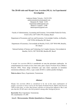
Figure 2 presents the distribution of answers subjects gave when they had to choose
between the hypothetical survey options of Rs. 300 in 1 month and a larger amount in 2
months. The figures show the fraction selecting each of the 4 possible answers to this
question. The bars are indexed by the delayed amount subjects would require to be
14
willing to wait. Thus, the bars further to the right correspond to participants who are
more willing to delay gratification. 18
60.0%
Figure 2: Distribution of Hypothetical Choices between
300 Rs in 1 Month and Larger Amount in 2 Months
50.0%
40.0%
30.0%
20.0%
Control
Treatment
10.0%
0.0%
> $495
$495
$375
$330
Minimum amount needed to be willing to delay until month 2.
Note: The figure shows the distribution of choices in a task in which subjects had to make
hypothetical choices between 300 Rs in 1 month and a larger amount in 2 months. The
horizontal axis shows the amount that was required for subjects to be willing to delay 300
Figure 2 and Appendix Figure 8 (which shows the same patterns for the today vs. 1
month condition) show the treatment group was more willing than the control group to
accept delayed payments in the hypothetical intertemporal choice task. In both figures
the mass of distribution of the treatment group is shifted to the right relative to the
distribution of the control group.
Table 4 confirms these results. The treatment is roughly 5 percentage points more
likely than the control group to be willing to give up Rs. 300 in 1 month in exchange for
18
Appendix Figure 8 presents the distribution over the four possible choices when subjects had to choose
between Rs. 200 today and a larger amount in 1 month.
15
Rs. 330 in 2 months (randomization-inference p-value = 0.06). Testing the full
distribution of choices in the two hypothetical tasks using a Wilcoxon rank-sum test, we
find randomization inference p-values for one-sided tests of 0.097 and 0.041
respectively (see Table 7), suggesting again that the null that the two groups have the
same choice patterns are rejected with at least marginal statistical significance.
Table 4: Treatment Effects on Hypothetical Intertemporal Choices
Choices
Cumulative Distribution of Choices
Control
Treatment
P-value
Standard
Mean
Effect
Random. Inf.
Error
Panel A: Choice between 300 Rs in 1 Month (sooner) and Larger Amount in 2 Months (later)
Willing to delay for at least 330 Rs
50.3%
5.3%
0.023
0.06
Willing to delay for at least 375 Rs
69.7%
-0.5%
0.85
Willing to delay for at least 495 Rs
87.8%
-0.5%
0.031
0.000
0.020
0.000
Unwilling to delay for 495 Rs
100.0%
0.78
Panel B: Choice between 200 Rs Today (sooner) and Larger Amount in 1 Month (later)
Willing to delay for at least 220 Rs
50.1%
5.8%
0.031
0.03
Willing to delay for at least 250 Rs
73.3%
1.6%
0.029
0.51
Willing to delay for at least 330 Rs
86.6%
-0.7%
0.022
0.000
0.72
Unwilling to delay for 330 Rs
100.0%
Note : The table reports the distribution of choices in two hypothetical intertemporal choice tasks. Panel A
reports the choices in a task in which subjects chose between receiving 300 rupees in 1 month and a larger
amount in 2 months. Panel B reports the choices in a task in which subjects chose between receiving 200 rupees
today and a larger amount in 1 month. The choices in this intertemporal choice tasks allow one to rank subjects
according to their willingness to delay gratification. For example, in Panel A subjects who chose 300 in 1 month
over 495 in 2 months were the least willing to accept a delayed payment while those who chose 330 in 2 months
over 300 in 1 month were the most willing to accept a delayed payment. The standard errors are clustered at the
village level and corrected for small sample (they are blown up by a factor of √(19/18) as recommended by
Cameron, Gelbach and Miller 2008) while the reported p-values are calculated using (nonparametric)
randomization inference (Rosenbaum 2002).
3.3. Incentivized CTB Choices
Figure 3 shows for each game the distribution of choices in the CTB experimental
task, separately for the control and treatment groups. Four sets of two bars are
16
presented. Each set corresponds to one of the four games; the left bar in each set
corresponds to the distribution of choices among the control group while the right bar
corresponds to the distribution of choices among the treatment group. Each bar contains
two parts: a blue part that is above the x-axis and a red part that is below the x-axis. The
blue part corresponds to the fraction of participants who were the most willing to delay
gratification, choosing to delay the maximum amount of Rs. 150 (Rs. 50 sooner). The
red part corresponds to the fraction of participants who were the least willing to delay
gratification, delaying the minimum amount of Rs. 50 (Rs. 150 sooner). 19 Thus, an
increase in the willingness to delay gratification corresponds to an increase in the blue
bar and/or a reduction in the red bar.
19
The fraction choosing the middle allocation can be inferred from the other two fractions.
17
The differences in choices across games reflect changes in the parameters of the
intertemporal choice across the games. In game 1 the experimental interest rate was
10%, the sooner date was “today” and the later date was “in 1 month.” The sooner date
was changed from “today” to “in 1 month” between games 1 and 2, while the time
interval between the sooner and later dates and the experimental interest rate were held
constant. Thus, present-biased individuals should be more willing to delay gratification
in game 2 than in game 1. Games 2 and 3 had the same time frame (sooner date “in 1
month”; later date “in 2 months”), but the interest rate was increased from 10% in game
2 to 20% in game 3. Individuals who are more responsive to interest rates (i.e., a higher
intertemporal elasticity of substitution) would be the ones to reallocate more money to
the later date in response to a change in the interest rate. Finally, the time delay was
increased from one month in game 3 to five months in game 4. While the sooner date
was the same in games 3 and 4 (“in 1 month”), the later date was “in 2 months” in game
3 and “in 6 months” in game 4 (the interest rate was held at 20% between games 3 and
4). Individuals with a higher discount rate would reallocate more resources to the sooner
date in response to an increase in the time delay.
The comparison of choices across games suggests that participants understood this
more complicated experimental task. For example, subjects re-allocate significantly
more money to the later date when the experimental interest rate is increased from game
2 to game 3. Subjects also reallocate more money to the sooner date when the delay
time is increased from game 3 to game 4. Interestingly, we see no evidence of present
bias. The choices in games 1 and 2 are very similar, even though the sooner date is
“today” in game 1 and “in 1 month” in game 2. Andreoni and Sprenger (2012) also
found no evidence of present bias when they conducted the CTB task with
undergraduate students. The results of Augenblick et al. (2013) suggest that tasks
involving choices over monetary rewards may be less suited to capture present bias than
tasks involving choices over real-effort-tasks.
We turn now to the treatment-control differences. Figure 3 shows that while the
choice patterns were broadly similar, the treatment group showed somewhat more
18
willingness to delay gratification. The treatment group is more likely to delay the
maximum amount possible of Rs. 150 and less likely to delay the minimum amount
possible of Rs. 50 (with the exception of game 2).
Table 5 reproduces the results presented graphically in Figure 3. Virtually none of
the differences are statistically significant, though most of the point estimates go in the
direction of more patience for the treatment group. In game 1 the treatment is 3.6
percentage points more likely than the control to delay the maximum possible of Rs.
150. In game 3 the treatment was roughly 5 percentage points more likely to delay the
maximum amount possible. This difference is marginally statistically significant with a
p-value of 0.07. The treatment group is also 2 and 4 percentage points less likely to
delay the smallest amount possible in games 3 and 4, respectively.
Table 5: Treatment Effects on Convex Time Budget Choices
Game
Control
Mean
Treatment
Effect
Standard Error
P-value
Random. Inf.
Panel A: Fraction Delaying Maximum Amount Possible (Sooner Reward = 50)
Game 1
50.5%
3.6%
0.031
0.23
Game 2
51.9%
0.4%
0.89
Game 3
64.0%
5.2%
0.032
0.000
0.037
0.000
0.07
Game 4
52.8%
-0.6%
0.036
0.84
Panel B: Fraction Delaying Minimum Amount Possible (Sooner Reward = 150)
Game 1
25.6%
0.0%
Game 2
22.5%
3.7%
Game 3
17.4%
-1.6%
Game 4
28.7%
-3.9%
0.028
0.000
0.029
0.000
0.024
0.000
0.024
1.00
0.16
0.46
0.15
Note : The table reports the distribution of choices in the adapted Convex Time Budget (CTB) task.
Panel A reports the fraction of subjects who were the most willing to accept a delay payment; they
chose a sooner reward of 50 rupees and delayed the maximum amount possible. Panel B reports the
fraction of subjects who were the least willing to accept a delay payment; they chose a sooner reward
of 150 rupees and delayed the minimum amount possible. The standard errors are clustered at the
village level and corrected for small sample (they are blown up by a factor of √(19/18) as recommended
by Cameron, Gelbach and Miller 2008) while the reported p-values are calculated using (nonparametric)
randomization inference (Rosenbaum 2002).
19
Next, we investigate whether treatment and control groups respond differently to
changes in the parameters of the experimental task, which may give us further insight
into any differences in the willingness to delay gratification between the two groups.
For this purpose, we compare how the allocations of treatment and control groups
change between: i) games 1 and 2 (change in the sooner date); ii) games 2 and 3
(change in the experimental interest rate); and iii) games 3 and 4 (change in time delay).
The results are shown in Table 6.
Table 6: Do Treatment and Control Respond Differently
to Changes in the Parameters of the Convex Time Budget (CTB) Task?
Changes in the Parameters of the
Intertemporal Choice
Control
Mean
Treatment
Effect
Standard
P-value
Error
Random. Inf.
Panel A: Increase in Fraction Delaying Maximum Amount Possible (Sooner Reward = 50)
Changing sooner date from today to a month later
1.5%
-3.1%
4.7%
0.027
0.000
0.045
0.000
Increase in interest rate from 10% to 20%
12.1%
Increase in time delay from 1 month to 5 months
-11.2%
0.40
0.17
-5.8%
0.044
0.12
Panel B: Increase in Fraction Delaying Minimum Amount Possible (Sooner Reward = 150)
Changing sooner date from today to a month later
-3.1%
3.7%
0.022
0.25
Increase in interest rate from 10% to 20%
-5.1%
-5.3%
0.038
0.07
Increase in time delay from 1 month to 5 months
11.3%
-2.2%
0.030
0.47
Note: The table investigates whether treatment and control groups respond differently to changes in the parameters of the
intertemporal choice task, namely the sooner date, the experimental interest rate, and the time interval between the sooner
and later dates. Panel A reports the increase in the fraction of subjects most willing to accept a delay payment across two
subsequent games. Panel B reports the increase in the fraction of subjects the least willing to accept a delay payment
across two subsequent games. From game 1 to game 2, the sooner date was changed from "today" to "in 1 month." From
game 2 to game 3 the experimental interest rate was increased from 10% to 20%. Finally, from game 3 to game 4 the time
delay between the sooner and later payments was increased from 1 month to 5 months. The standard errors are clustered
at the village level and corrected for small sample (they are blown up by a factor of √(19/18) as recommended by Cameron,
Gelbach and Miller 2008) while the reported p-values are calculated using (nonparametric) randomization inference
(Rosenbaum 2002).
We find the treatment group is more responsive than the control group to an
increase in the experimental interest rate. When the experimental interest rate increases
from 10% to 20%, there is a 12 percentage points increase in the fraction of control
choosing to delay the maximum amount and a 17 percentage points increase among the
20
control. Similarly, the increase in experimental interest rates leads to a 5 percentage
points decrease in the fraction of the control choosing to delay the minimum amount
and a 11 percentage points reduction among the treatment. This difference is
statistically significant at 10%. There is some weak evidence, though not statistically
significant, that the control reacts more to going from immediate to delayed payments
from Game 1 to 2 in a way that would suggest the control group may show some
present bias while the treatment does not. Finally, the evidence on which group is more
responsive to the increase in the time delay is mixed.
Overall, the reduced-form results show that the treatment group is more responsive
to an increase in the experimental interest rate, which suggests that the treatment group
may be more willing to delay gratification because it has a higher intertemporal
elasticity of substitution. This hypothesis is also consistent with the evidence that the
treatment group is more likely to choose riskier options in the lottery choice task. In
fact, in models with constant-relative-risk-aversion (CRRA) risk preferences, which are
commonly used in the literature, a higher intertemporal elasticity of substitution
corresponds to a less concave and more risk-neutral utility function.
3.4 Differences Combining Outcomes and Tasks
The differences in the average choices of treatment and control in all three
experimental tasks have the expected sign (with some exceptions in the CTB task) but
are often only marginally statistically significant.
These effects likely represent a
combination of moderate effect sizes and somewhat sizeable standard errors. The
moderate effect sizes for this experiment that randomized access to savings are not
particularly surprising when one considers that there are likely a range of influences
beyond savings that affect risk and intertemporal-choice attitudes.
The need for
simplicity also led us to keep the choice tasks to a relatively limited set of discrete
options that could be displayed visually, which likely also affects the power we have in
detecting average choice differences. It is also worth noting that the estimated treatment
effects are intent-to-treatment estimates and the difference in magnitudes would be even
21
larger if one took into account that one-fifth of the treatment group declined the offer to
open a savings account.
To address the broader question of whether access to savings has some effect on
attitudes toward risk and intertemporal tradeoffs it is possible to step back from looking
at differences in average choice frequencies and consider the distribution of choices
more broadly. Imbens and Wooldridge (2009) argue that combining rank-sum tests
with randomization-inference for the p-values (ala Rosenbaum, 2002) is an important
method for determining whether observed patterns in randomized experiments imply
that the treatment had some effect on the outcome of interest. In Table 7 we show the
p-values from Wilcoxon rank-sum tests of differences between treatment and control
for each task and combinations of the different experimental tasks. Combining all tasks
we see a p-value of 0.03 on the test of equality between treatment and control,
providing clear evidence of differential choice patterns overall for those given access to
savings accounts.
Table 7: P-values for Wilcoxon Rank-sum Tests
Tests of equality in single tasks
Experimental task
Risk game
Hypothetical intertemporal — today vs one month
Hypothetical intertemporal — one month vs two months
CTB game 1 — today vs 1 month and r = 10%
CTB game 2 — 1 month vs 2 months and r = 10%
CTB game 3 — 1 month vs 2 months and r = 20%
CTB game 4 — 1 month vs 6 months and r = 20%
p-value
0.10
0.04
0.10
0.30
0.38
0.01
0.32
Tests of equality across multiple tasks
Combined tasks
p-value
Hypothetical intertemporal (two delays combined)
0.05
CTB (all 4 games combined)
0.09
Risk + Hypothetical intertemporal
0.03
Risk + CTB
0.07
Hypothetical intertemporal + CTB
0.03
All tasks combined
0.03
Note: The table reports the p-values for one-sided Wilcoxon rank-sum tests (Wilcoxon 1945) computed using (nonparametric) randomization inference
(Rosenbaum 2002). The left-hand columns show p-values for individual tasks. The right-hand columns show p-values for combined tasks. The sharp null
hypothesis is that the outcomes of every study participant would have remained the same if the participant’s treatment status was switched. The null
hypothesis is rejected with a confidence level of 1-α if the observed Wilcoxon statistic is in the α% upper tail of the distribution (variables in which the
observed ranks of treatment were smaller than the observed ranks of control were multiplied by -1). The rank sum is calculated separately for each one of the
19 strata and then summed over strata. In the tests across multiple tasks the rank-sum is calculated separately for each task and then aggregated over tasks
(Rosenbaum 1997).
4. Potential Mechanisms and Structural Estimation
Section 3 documented that treatment and control make different choices in the
experimental tasks, remaining agnostic about what may underlie these differences in
22
behavior. In this section we discuss two broad mechanisms through which access to
savings accounts could affect risk-taking and intertemporal choice behavior. One
potential mechanism is the “wealth effect”. As discussed in section 2.1, the savings
account enabled the treatment group to accumulate more wealth than the control group,
which may have changed their marginal utility of consumption in ways that could affect
their choices in the experimental tasks. The alternative mechanism is that gaining access
to savings accounts may have changed preferences more broadly. Such changes in
preferences could reflect changes in how easily one envisions the future, how aware one
is of the broader impacts of immediate choices, and different emotional responses to
windfall income. It is both conceptually and empirically challenging to disentangle
potential wealth effects from preference changes, but here we provide some suggestive
evidence about the potential mechanisms.
4.1 Wealth, Background Consumption and Narrow Bracketing
The first step to exploring potential wealth effects versus broader preferencechange mechanisms is to establish what might be meant by wealth effects.
As
Andersen et al. (2008) highlight, there has historically been a fair amount of confusion
on this point in the literature. While it is common to think of wealth as simply a stock
of money, recent work has clarified that models of economic preferences are based on
the concept that individuals maximize their utility of consumption, with income and
wealth forming the budget constraint (Chetty, 2006; Andersen et al. 2008). The key
issues in exploring the effects different levels of wealth may have on choices in
experimental tasks are first, understanding how wealth differences map into
“background” consumption differences over time and second, understanding the extent
to which individual choices in experimental tasks come from a choice process that is
integrated with background consumption.
To address the first of those questions we explore how the increased wealth
available to the treatment group in their savings accounts is likely to differentially affect
the background consumption profiles of treatment and control groups. The savings
23
experiment clearly impacted the available assets of the treatment group. However, the
data suggest that – around the time the experimental tasks were administered – these
greater assets did not translate into substantial differences in the average level of
consumption of the control and treatment groups. Administrative bank data show that a
year after the introduction of the program the average and median savings account
balances had roughly plateaued. Savings-account participants continued to make
deposits and withdrawals, but the two had roughly balanced each other out, suggesting
that on average the treatment group was neither increasing saving nor dissaving. 20
Moreover, as Prina (2013) discusses, the savings experiment did not change the income
level of the treatment group. The combination of these two patterns suggests that the
average weekly expenditures were likely similar for the two groups around the time our
data were collected.
Although additional wealth did not fundamentally change
consumption levels for the treatment group, their savings give them an additional
buffer. Having some buffer wealth may have allowed treatment households to smooth
consumption, transferring resources from good times to lean times and keeping a flatter
profile of background consumption. To summarize, then, we expect that access to
savings likely resulted in roughly equal levels of background consumption but may
have reduced the variance of background consumption for the treatment group relative
to control.
The second issue is to address how background consumption affects how
individuals make choices in the experimental tasks. One approach is to assume that
experimental choices come from a utility model that is independent of background
consumption utility. We label this possibility the “extreme narrow bracketing” case,
and note that a number of papers document that individuals make choices, especially in
experimental tasks, while appearing to largely ignore other circumstances they face
20
These figures were calculated using GONESA bank’s administrative data on the savings account
balance, deposits and withdrawals of treatment households.
24
(Tversky and Kahneman 1981, Rabin and Weizsacker 2009). 21 The utility framework
most consistent with the extreme narrow bracketing possibility is prospect theory
(Kahneman and Tversky, 1979). 22
In this type of framework individuals make
experimental choices based on how they feel about the outcomes (i.e., changes in
wealth) from those choices in isolation. Under the extreme narrow bracketing
assumption, then, there is no clear role for wealth to directly affect choices through the
marginal utility of consumption, and hence it would be natural to interpret differences
as coming from broader effects on preferences.
A second approach is to take seriously the effects of background consumption
and assume that individuals make choices in experiments anticipating integrating their
experimental rewards with their background consumption (Andersen et al, 2008). This
is the assumption that is most consistent with the dominant expected-utility paradigm.
Within this approach we can label two further sub-cases, which are formalized and
discussed in detail by Andersen et al. (2008). The first is what we call the “integrated
and immediately consumed” case, in which one assumes that subjects make
experimental choices anticipating adding their experimental reward when received to
their background consumption at that time. The second possibility is what we call the
“integrated and re-optimized” case, in which the subjects make experimental choices
anticipating that they will fully re-optimize their consumption stream to include the
experimental rewards. As a number of authors have highlighted (e.g., Rabin 2000,
Schechter, 2007, Andersen et al., 2008), the “integrate and re-optimize” case is
generally not supported by experimental data as it predicts that individuals will be
essentially risk neutral and largely completely patient when faced with the vast majority
21
There is also a very closely related literature on “myopic loss aversion” that discusses how forms of
narrow bracketing help to explain various phenomena such as the equity premium puzzle (e.g., Benartzi
and Thaler 1995, Gneezy and Potters 1997).
22
As Andersen et al. (2008) point out, many experimental papers estimate utility functions using this
extreme narrow bracketing assumption, though most do so without reference to the explicit assumption
and maintain an expected-utility-of-consumption framework that is not consistent with the formal
modeling.
25
of monetary choices in experimental settings. 23 As such, for this paper we focus on
structural estimation under both the “extreme narrow bracketing” and “integrated and
immediately consumed” cases. 24
Before turning to the structural estimation, we note that we have some
suggestive evidence that would favor the narrow bracketing assumption. There was
some likely natural variation in background circumstances for individuals depending on
the date when our evaluators reached the household to administer these tasks. The tasks
happened to be administered around the Dashain, Nepal’s most important national
holiday, which in 2011 happened between October 3rd and October 12th. Because
households incur major expenses associated with the Dashain festivities, we expect that
the Dashain would generate large variations in levels of background consumption and
cause potential liquidity constraints for the households without savings. 25 Thus, if
subjects were integrating their background consumption, we would expect to see
differences between the experimental choices of subjects who played the experimental
tasks closer to the Dashain and the experimental choices of subjects who played them
farther from the Dashain.
Figure 4A shows the relationship between self-reported household savings and
the date at which the experimental tasks were administered for the control group. The
section of the graph between October 3rd and October 12th has no data and corresponds
to the Dashain, when no interviews were conducted. There is a strong negative
relationship between self-reported savings levels and the proximity to the Dashain: in
23
Consistent with the preceding literature, our subjects display meaningful risk aversion over modest
stakes and fail to take advantage of available arbitrage opportunities inherent in the CTB task that had a
much higher experimental interest rate than available in the market. Both of these facts are inconsistent
with models of fully sophisticated asset integration and re-optimization.
24
Andersen et al. (2008) present a method for incorporating intermediate cases of re-optimization for
experimental tasks and exploit differential timing of receipt of rewards between lottery tasks and
intertemporal choices. In our experiment, since the lottery tasks were paid with vouchers that could be
collected along with the intertemporal payouts, we suspect that the underlying assumptions of the
Andersen et al. (2008) approach are less likely to hold with our payout structure than with the methods
they employed.
25
A household would spend money among other things buying new clothes and animals like goats and
chickens to be slaughtered as religious sacrifices.
26
roughly 30 days the average savings (from all sources) fell from approximately Rs.
60,000 all the way to Rs. 5,000. 26
Note: The figures plot the average savings (A), the fraction of participants who chose the largest today rewards of Rs. 150
(B) and the fraction who chose the risk-free lottery (C) among the control group who were administered the experimental
tasks at a given day. The balls’ circumferences correspond to the mass of participants surveyed at the given day.
If individuals were integrating, one might expect less willingness to delay
gratification and less willing to take risks as it got closer to the holiday and they became
increasingly liquidity constrained. However, the data do not support this hypothesis.
Figure 4B plots the fraction of participants who chose in game 1 to receive the largest
sooner reward of Rs. 150, which they could redeem on the same day, against the
interview date. There is no evidence that individuals were less willing to delay
gratification as it got closer to the holiday. Figure 4C is consistent with Figure 4B,
showing that individuals were no more likely to choose the risk-free option in the
lottery-choice task as the holidays approached.
26
The results are qualitatively the same if one controls for baseline wealth or calculates median (rather
than mean) savings per day.
27
4.2 Structural Model
The proceeding section makes it clear that it is an open question as to whether the
observed choice patterns reflect wealth effects or some type of preference change. In
order to better explore the implications our findings have for understanding preference
change, we turn to a structural utility model. This approach allows us to ask for
different assumptions about the effects of background wealth, and holding fixed the
preference model, the question: How different would the preference parameters of the
28
control and treatment groups have to be to generate the experimental task choices we
observe in the data?
The interpretation of the estimates from this structural-estimation exercise differs
somewhat depending on whether we consider the “extreme narrow bracketing” or the
“integrate and immediately consume” case. Under extreme narrow bracketing, there are
no differences in background consumption that get incorporated into the utility model,
and hence any differences in choice patterns load on the utility model’s preference
parameters.
In the “integrated and immediately consumed” case we explicitly
incorporate different assumptions about how gaining access to savings accounts may
have affected the treatment group’s background consumption. With this approach the
structural estimation reveals whether or not the treatment-control differences in
background consumption can fully rationalize the choice patterns without requiring
additional differences in preference parameters between the two groups.
Our investigation of these different approaches highlights that one should be
cautious when interpreting the results of the structural estimation. It is not clear which
assumptions are most valid, and more generally, any parsimonious utility model will
attribute a range of influences that are not captured by the model to the model’s
parameters. As such, estimated parameters do not necessarily reflect deep and specific
psychological constructs. Nonetheless, we see the value of structural estimation for
allowing us to better quantify effects and to more deeply explore the potential
implications the observed choice-pattern differences have for our understanding of
individual behavior.
4.2.1 Model
We begin by outlining the structural utility model that can be fit to the CTB task,
which allows us to jointly estimate present bias, exponential discount rates, and a riskaversion coefficient under a single unified framework.
We follow Andreoni and
Sprenger (2012) in modeling the intertemporal choice of an agent with time separable
utility and quasi-hyperbolic time preferences faces in the experimental task. In a given
29
game 𝑔𝑔 the agent must choose between receiving Rs. 150, 100 or 50 sooner. The later
reward, 𝐿𝐿𝐿𝐿𝑔𝑔 , is given by:
𝐿𝐿𝐿𝐿𝑔𝑔 = �200 − 𝑆𝑆𝑆𝑆𝑔𝑔 � ∗ 𝑅𝑅𝑔𝑔 ,
(1)
where 𝑆𝑆𝑆𝑆𝑔𝑔 is the sooner reward, and 𝑅𝑅𝑔𝑔 the gross experimental interest rate in game 𝑔𝑔.
Assuming that the agent has constant-relative-risk-aversion (CRRA) risk preferences,
the utility of a given allocation is given by:
1−𝜌𝜌
U�𝑆𝑆𝑆𝑆𝑔𝑔 , 𝐿𝐿𝐿𝐿𝑔𝑔 � = ��𝑆𝑆𝑆𝑆𝑔𝑔 + ω1 �
1−𝜌𝜌
+ βτ𝑔𝑔 δk𝑔𝑔 �𝐿𝐿𝐿𝐿𝑔𝑔 + ω2 �
� /[1 − 𝜌𝜌],
(2)
where the preference parameters are: 𝜌𝜌, the CRRA relative-risk-aversion coefficient; β,
the present bias; and δ, the monthly discount factor. The parameters of the game 𝑔𝑔
intertemporal choice are: τ𝑔𝑔 , an indicator variable that is 1 if the sooner date in game 𝑔𝑔
is today (and 0 otherwise); k𝑔𝑔 , the time delay (in months) between the sooner and later
dates; and 𝑅𝑅𝑔𝑔 is the gross experimental interest rate. The parameter ω1 is the
background consumption in the period in which the agent receives the sooner reward
and ω 2 is the background consumption in the period in which the agent receives the
later reward. We follow Andersen et al. (2008) in defining this background
consumption as “the optimized consumption stream based on wealth and income that is
[perfectly] anticipated before allowing for the effects of the money offered in the
experimental tasks.” 27 With these background consumption parameters in place, the
model corresponds to the “integrated and immediately consumed” case discussed in the
preceding sessions. If these parameters are set to zero, the model corresponds to the
“extreme narrow bracketing” case and the risk-aversion coefficient can be thought of as
an estimate of the curvature of the prospect-theoretic value function over gains.
It is easy to show that the agent chooses to receive 150 sooner if condition (3)
holds and chooses 50 sooner if condition (4) holds:
27
Notice there is an assumption, which is the standard in the literature, that the agent chooses the optimal
background consumption without taking the experimental rewards into account, such that the agent does
not re-optimize if there is any reallocation of the experimental rewards.
30
𝑙𝑙𝑙𝑙
𝑙𝑙𝑙𝑙
(150 + ω1 )1−𝜌𝜌 − (100 + ω1 )1−𝜌𝜌
1−𝜌𝜌
�100𝑅𝑅𝑔𝑔 + ω2 �
(100 + ω1 )1−𝜌𝜌 −(50 + ω1 )1−𝜌𝜌
1−𝜌𝜌
�150𝑅𝑅𝑔𝑔 + ω2 �
1−𝜌𝜌
> 𝑌𝑌𝑔𝑔∗ ,
(3)
1−𝜌𝜌
< 𝑌𝑌𝑔𝑔∗ ,
(4)
− �50𝑅𝑅𝑔𝑔 + ω2 �
− �100𝑅𝑅𝑔𝑔 + ω2 �
where 𝑌𝑌𝑔𝑔∗ = τ𝑔𝑔 lnβ + k𝑔𝑔 lnδ is the effective discount factor in game 𝑔𝑔 in logs. If neither
condition (3) nor (4) holds, the agent chooses to receive 100 sooner.
In taking the model to the data, we assume an addictive error structure:
∗
𝑌𝑌𝑖𝑖,𝑔𝑔
= τ𝑔𝑔 lnβ + k𝑔𝑔 lnδ + 𝜀𝜀𝑖𝑖,𝑔𝑔 ,
(5)
where 𝜀𝜀𝑖𝑖,𝑔𝑔 is an error term that is specific to individual 𝑖𝑖 and game 𝑔𝑔 and is normally
distributed with mean zero and variance 𝜎𝜎 2 —i.e., 𝜀𝜀𝑖𝑖,𝑔𝑔 ~ N(0,𝜎𝜎 2 ). Under these
assumptions, the likelihood of individual 𝑖𝑖’s choice in game 𝑔𝑔 is given by: 28
(100+ω )1−ρ
ℒ𝑖𝑖,𝑔𝑔 =
)1−ρ
−(50+ω1
lnβ
lnδ
1
⎧ 1 − Φ � 1 𝑙𝑙𝑙𝑙
τ𝑔𝑔 −
k � if 𝑆𝑆𝑆𝑆𝑖𝑖,𝑔𝑔 = 50,
1−ρ
1−ρ −
𝜎𝜎
𝜎𝜎
𝜎𝜎 𝑔𝑔
+ω
−�100𝑅𝑅
+ω
�150𝑅𝑅
�
�
𝑔𝑔
2
𝑔𝑔
2
⎪
⎪
(100+ω1 )1−ρ −(50+ω1 )1−ρ
1
lnβ
lnδ
τ − k𝑔𝑔 � −
Φ � 𝑙𝑙𝑙𝑙
⎪
1−ρ
1−ρ −
𝜎𝜎
𝜎𝜎 𝑔𝑔
𝜎𝜎
�150𝑅𝑅𝑔𝑔 +ω2 �
−�100𝑅𝑅𝑔𝑔 +ω2 �
(150+ω1 )1−ρ −(100+ω1 )1−ρ
1
lnβ
lnδ
⎨
τ −
k �
−Φ � 𝑙𝑙𝑙𝑙
1−ρ
1−ρ −
𝜎𝜎
𝜎𝜎 𝑔𝑔
𝜎𝜎 𝑔𝑔
⎪
−�50𝑅𝑅𝑔𝑔 +ω2 �
�100𝑅𝑅𝑔𝑔 +ω2 �
⎪
⎪Φ � 1 𝑙𝑙𝑙𝑙 (150+ω1 )1−ρ −(100+ω1 )1−ρ − lnβ τ − lnδ k �
1−ρ
1−ρ
𝜎𝜎
𝜎𝜎 𝑔𝑔
𝜎𝜎 𝑔𝑔
−�50𝑅𝑅𝑔𝑔 +ω2 �
�100𝑅𝑅𝑔𝑔 +ω2 �
⎩
(6)
if 𝑆𝑆𝑆𝑆𝑖𝑖,𝑔𝑔 = 100,
if 𝑆𝑆𝑆𝑆𝑖𝑖,𝑔𝑔 = 150.
Using (6) we estimate the variance of the error term 𝜎𝜎 2 and separate preference
parameters (δ, 𝛽𝛽, 𝜌𝜌) for the control and treatment groups via maximum likelihood. The
variance of the error term is assumed to be the same for the two groups.
We follow an analogous approach to map the lottery-choice data into an estimate of
risk aversion. Specifically, we assume that an agent with constant-relative-risk-aversion
risk preferences must choose among five lotteries with payouts dependent on a coin
toss. We use 𝑙𝑙 to index a lottery 𝔏𝔏𝑙𝑙 = (ℎ𝑙𝑙 , 𝑡𝑡𝑙𝑙 ) that paid ℎ𝑙𝑙 if the coin landed on heads
and 𝑡𝑡𝑙𝑙 if it landed on tails:
𝔏𝔏1 = (20,20), 𝔏𝔏2 = (30,15), 𝔏𝔏3 = (40,10), 𝔏𝔏4 = (50,5), 𝔏𝔏5 = (55,0).
28
Andreoni et al. (2012) adopt an alternative approach and use interval-censored Tobit to estimate
preference parameters when the Convex Time Budget task involves a choice between few options.
31
The utility of a lottery 𝔏𝔏𝑙𝑙 is given by:
U( 𝔏𝔏𝑙𝑙 ) =
1 (ℎ𝑙𝑙 + ω)1−𝜌𝜌 1 (𝑡𝑡𝑙𝑙 + ω)1−𝜌𝜌
+
,
1 − 𝜌𝜌
2 1 − 𝜌𝜌
2
(7)
where 𝜌𝜌 is the CRRA risk aversion parameter and ω is the background consumption in
the period in which the agent receives the experimental reward.
It is easy to show that the agent chooses lottery 𝑙𝑙 = 1 if (8) holds and 𝑙𝑙 = 5 if (9)
holds. The agent chooses 𝑙𝑙 = 2,3, or 4 if both (8) and (9) hold:
𝑙𝑙𝑙𝑙
(ℎ𝑙𝑙 + ω)1−𝜌𝜌 − (ℎ𝑙𝑙−1 + ω)1−𝜌𝜌
> 𝑍𝑍 ∗ > ln
(𝑡𝑡𝑙𝑙−1 + ω)1−𝜌𝜌 − (𝑡𝑡𝑙𝑙 + ω)1−𝜌𝜌
𝑙𝑙𝑍𝑍 ∗ > 𝑙𝑙𝑙𝑙
where 𝑍𝑍 ∗ = 0.
, (8)
(ℎ𝑙𝑙+1 + ω)1−𝜌𝜌 − (ℎ𝑙𝑙 + ω)1−𝜌𝜌
,
(𝑡𝑡𝑙𝑙 + ω)1−𝜌𝜌 − (𝑡𝑡𝑙𝑙+1 + ω)1−𝜌𝜌
(9)
In taking the model to the data, we assume an addictive error structure:
𝑍𝑍𝑖𝑖∗ = 𝜉𝜉𝑖𝑖 ,
(10)
where 𝜉𝜉𝑖𝑖 is an error term that is specific to individual 𝑖𝑖 and is normally distributed with
mean zero and variance 𝜂𝜂2 —i.e., 𝜉𝜉𝑖𝑖 ~ N(0,𝜂𝜂2 ). Under these assumptions, the likelihood
of individual 𝑖𝑖’s choice is given by:
ℒ𝑖𝑖 =
⎧
⎪
⎪
⎪
⎨
⎪
⎪
⎪
⎩
1 − Φ�
Φ�
1−𝜌𝜌
𝑙𝑙
𝑙𝑙+1
1−𝜌𝜌
1−𝜌𝜌
�ℎ𝑙𝑙 +ω�
−�ℎ𝑙𝑙−1 +ω�
1−𝜌𝜌
1−𝜌𝜌 � −
−�𝑡𝑡𝑙𝑙 +ω�
�𝑡𝑡𝑙𝑙−1 +ω�
1−𝜌𝜌
1−𝜌𝜌
�ℎ𝑙𝑙+1 +ω�
−�ℎ𝑙𝑙 +ω�
1
�
−Φ �
1−𝜌𝜌
1−𝜌𝜌
𝜎𝜎
−�𝑡𝑡𝑙𝑙+1 +ω�
�𝑡𝑡𝑙𝑙 +ω�
1
𝑙𝑙𝑙𝑙
𝜂𝜂
Φ�
1−𝜌𝜌
�ℎ
+ω�
−�ℎ𝑙𝑙 +ω�
1
𝑙𝑙𝑙𝑙 𝑙𝑙+1 1−𝜌𝜌
1−𝜌𝜌 �
𝜂𝜂
−�𝑡𝑡 +ω�
�𝑡𝑡 +ω�
𝑙𝑙𝑙𝑙
1−𝜌𝜌
1−𝜌𝜌
�ℎ +ω�
−�ℎ𝑙𝑙−1+ω�
1
𝑙𝑙𝑙𝑙 𝑙𝑙
1−𝜌𝜌
1−𝜌𝜌 �
𝜂𝜂
+ω�
−�𝑡𝑡 +ω�
�𝑡𝑡
𝑙𝑙−1
𝑙𝑙
4.2.2 Structural Estimates Assuming Narrow Bracketing
if 𝑙𝑙 = 1,
(11)
if 𝑙𝑙 = {2,3,4},
if 𝑙𝑙 = 5.
Table 8 presents the results from the structural estimation. Panel A shows the
estimates of the annual discount factor (δ), relative risk aversion (ρ), and present bias
(β) based on choices in the CTB task. Panel B shows a separate estimate of relative risk
32
aversion (ρ) from the lottery-choice task. In each case we show the parameter estimate
obtained for the control group and the ratio of the treatment group’s estimate to that of
control.
Table 8: Maximum Likelihood Estimation of Preference Parameters
Background Consumption
Control group:
ω1 = 0
ω2 = 0
ω 1 = 300
ω 2 = 300
Ν(300,225)
Ν(300,3600)
ω 1 = 285
ω 2 = 300
ω 1 = 300
ω 2 = 300
Treatment group:
ω1 = 0
ω2 = 0
ω 1 = 300
ω 2 = 300
ω 1 = 300
ω 2 = 300
ω 1 = 300
ω 2 = 300
ω 1 = 300
ω 2 = 300
ω 1 = 292.5
ω 2 = 307.5
Panel A: Convex Time Budget Task
Parameter Estimates
Annual Discount Factor Control (δ)
Discount Factor Treatment / Discount Factor Control
Risk Aversion Control (ρ)
Risk Aversion Treatment / Risk Aversion Control
Present Bias Control (β)
Present Bias Treatment / Present Bias Control
Hypothesis Tests (P-Values)
Test Difference in Annual Discount Rates
Test Difference in Risk Aversion
Test Difference in Present Bias
Joint Test Differences in Preference Parameters
ω1, ω2 distributed as
(n = 4,420)
0.79
(0.022)
1.02
(0.037)
0.12
(0.008)
0.93
(0.066)
1.00
(0.009)
1.01
(0.013)
0.79
(0.021)
1.02
(0.037)
0.45
(0.030)
0.94
(0.067)
1.00
(0.009)
1.01
(0.013)
0.79
(0.021)
1.02
(0.037)
0.45
(0.030)
0.94
(0.067)
1.00
(0.009)
1.01
(0.013)
0.79
(0.021)
1.02
(0.037)
0.44
(0.029)
0.96
(0.068)
1.00
(0.009)
1.01
(0.013)
0.82
(0.022)
0.97
(0.033)
0.42
(0.026)
0.97
(0.068)
1.01
(0.009)
1.00
(0.012)
0.78
(0.020)
1.06
(0.037)
0.43
(0.028)
0.92
(0.065)
1.00
(0.009)
1.02
(0.013)
0.67
0.32
0.57
0.65
0.67
0.33
0.57
0.65
0.67
0.34
0.57
0.66
0.67
0.56
0.57
0.82
0.34
0.62
0.71
0.79
0.10
0.23
0.16
0.08
Panel B: Lottery Choice Task (n = 1,105)
Parameter Estimates
Risk Aversion Control (ρ)
Risk Aversion Treatment / Risk Aversion Control
Hypothesis Test (P-Value)
Test Difference in Risk Aversion
0.40
(0.026)
0.95
(0.062)
6.82
(0.384)
0.95
(0.053)
6.73
(0.374)
0.96
(0.053)
5.65
(0.282)
1.14
(0.059)
6.51
(0.366)
0.99
(0.055)
6.82
(0.384)
0.92
(0.051)
0.38
0.30
0.43
0.02
0.88
0.14
Note: The table shows Maximum Likelihood estimates of preference parameters under different assumptions about background consumption. Panel A reports results estimated using
choices in the Convex Time Budget task while Panel B reports results estimated using the choices in the lottery-choice task. The first column is the "narrow bracketing" case and
assumes zero background consumption incorporated in the CTB and risk choices. The second column assumes a static level of background consumption of 300 rupees for everyone in
both the treatment and control group in both periods. The third and fourth columns assume the control had uncertainty about their background consumption and it is assumed that
their background consumption followed a normal distribution (the background consumption of treatment is held constant at 300 rupees). The last two columns consider an upward
slope of consumption for control and treatment respectively. Standard errors in parenteshes are clustered at the individual level in Panel A and clustered at the village level in Panel B .
The bottom portion of the panels shows p-values from tests that the parameters for
treatment and control are the same. The standard errors on these structural parameter
estimates are sizeable and throughout this table we fail to detect statistically significant
differences between treatment and control. This likely reflects a combination of the
33
discrete choice set we used in the CTB task, which reduced the variation available for
parameter estimation relative to the continuous version, moderate underlying choicepattern effects, and inherent noise in the experimental data.
Despite the noise in the
estimates, however, we still see merit in exploring the point estimates from the
estimation. In our view there are two goals of the structural estimation. First, we hope
to provide a way of quantifying the potential implications of the choice patterns we
observe. Second, we aim to explore how the implications of the choice patterns for
preferences depend on assumptions about the integration of background wealth and
thereby speak to the question of wealth effects versus broader preference-change
mechanisms. As long as one remains cautious in interpreting the somewhat noisy
estimates, we feel both of these goals can be served by focusing on the point estimates
from the structural models.
The estimates in the first column of Table 8 give the narrow bracketing case, in
which ω1 = ω2 = 0. The control group is estimated to have an annual discount factor
of 0.79.
That suggests this population strongly discounts the future, but is not
implausible given that annual inflation in Nepal was above 10% during the study period
(IMF 2011). Interestingly, our estimates suggest less discounting of the future by the
Nepalese villagers than was observed by Andreoni and Sprenger (2012) when they
conducted the CTB with undergraduate students in the U.S. We obtain a CRRA
parameter in the narrow bracketing case for the control group of 0.12, which is similar
to the estimates Andreoni and Sprenger (2012) provide for their sample and corresponds
almost exactly to the original curvature estimated for the value function in gains for
prospect theory by Tversky and Kahneman (1992).
The results indicate the treatment group is more patient than the control group. The
estimated discount factor for the treatment group is 2 percent higher than that of the
control. Alternatively, the treatment group has an annual discount rate 2.5 percentage
points lower than the control. There is no present bias for the control or treatment,
which is consistent with the choice patterns.
34
We also find the treatment group is less risk averse than the control group. In the
CTB task, the estimated (coefficient of) relative risk aversion for the treatment group is
7 percent lower than that of the control. The estimates from the lottery-choice task
imply similar treatment-control differences in percentage terms. In the lottery-choice
task, the estimated (coefficient of) relative risk aversion for the treatment group is 5
percent lower. These results are again consistent with the choice patterns that suggested
more linear utility for the treatment.
However, the estimates of the level of the risk-aversion are different across
tasks. From the lottery-choice task, we obtain an estimate a coefficient of relative risk
aversion of 0.40 for the control group, substantially higher than that estimated from the
CTB task. This difference could reflect the challenges of fitting the simple CRRA
functional form over varying stakes, as the CTB task had outcomes that were 5 to 10
times the size of the lottery task. Andreoni and Sprenger (2012) find the same pattern,
with higher risk aversion measures in a multiple price list lottery task than in the CTB,
and posit that this may suggest that prospects with underlying risk have are governed in
part by an additional force beyond simple utility-of-outcome curvature.
4.2.3 Structural Estimates Assuming Asset Integration
Columns 2 through 6 present structural estimation results for different assumptions
about background consumption under the assumption that experimental rewards are
integrated with background consumption and immediately consumed when received. In
Column 2 we assume that all members of each group have daily background
consumption equal to Rs. 300, which is close to the typical daily income reported by
these households, and that the background consumption is constant over time.
Incorporating this level of background consumption increases the estimated riskaversion parameters significantly, especially for the lottery-choice task, but does not
change the other parameters or the estimates of the percentage differences between
treatment and control in a meaningful way.
35
Columns 3 and 4 represent our best attempt to incorporate the potential
differences in background wealth for treatment and control. For these columns we
assume that the treatment group has constant daily background consumption of Rs. 300.
The idea is that their buffer stock of savings may allow them to perfectly smooth
consumption over time. The control group, however, does not have this same buffer
stock and efficient saving device and hence may face variation in background
consumption.
In column 3 we assume that the control group’s daily background
consumption averages Rs 300 but is normally distributed with a variance of Rs. 225, or
a standard deviation of daily consumption of 5%. In column 4 we increase the standard
deviation of daily consumption to 20% for the control.
Comparing the results in Columns 3 and 4 to those in Column 2 we see that the
addition of background consumption risk for the control group can have strong effects
for the estimates from the lottery-choice task, but does relatively little to the estimates
from the CTB task. Risk aversion measured from the lottery choices falls substantially
for the control group as we add background risk. Moving from 5% to 20% standard
deviation in background consumption for the control we observe a switch from the
treatment group being estimated to have 4% lower risk aversion to treatment having
14% higher risk aversion. This result suggests to us that the observed differences in risk
aversion in the lottery task could be rationalized by the effects of background wealth on
consumption, if the access to savings accounts allows the treatment group to reduce the
standard deviation of their daily consumption by somewhere between 5% and 20%
relative to control. However, even substantial differences in background variation
(Colum 4) have very little impact in the CTB task and cannot drive away the modest
differences in either estimated discount factors or risk aversion for this task.
Although we believe the most likely effect of differential wealth accumulation
for the treatment group will come through reductions in the variance of consumption, in
Columns 5 and 6 we explore the possibility that the two groups might have differential
trends in background consumption. In Column 5 we investigate how the estimates
would change if we assumed the control group was temporarily liquidity constrained
36
when we conducted the experimental tasks and had “sooner” background consumption
5% lower than “later” background consumption. With this assumption the differential in
risk aversion parameters from the lottery task between treatment and control is
essentially eliminated and is reduced to 3% for the CTB task. However, with this
assumption the parameters yield the implication that the treatment group has an
estimated discount factor lower than that of the control, suggesting that they would be
somewhat less patient than the control. In Column 6 we explore a different possibility,
namely that the treatment group could have been engaged in continued asset building
during this period with the intention of increasing their daily consumption in the future.
We capture this by assuming a 5% differential in background consumption between the
two periods for the treatment group. In this case, all of the differentials in patience and
risk aversion between the two groups are significantly magnified and often marginally
statistically significant.
Taken all together, this exercise in exploring the effects of background
consumption on parameter estimates suggests to us that wealth effects could plausibly
account for some of the differences we observe in choice patterns under the assumption
of otherwise stable preferences between the two groups. However, it is difficult to find
background consumption differences that can rationalize the choice patterns across both
the lottery task and CTB task under the assumption that the two groups have the same
preferences. While this exercise is certainly not conclusive, it provides some suggestive
evidence that broader preference-change mechanisms could be at play in this
environment.
5. Conclusion
We exploited a field experiment that randomized access to savings accounts to
investigate whether attitudes toward risk and intertemporal choices are affected by the
act of saving. Because the majority of the sample had never had a savings account
before, the experiment generated random variation in savings behavior. A year later we
administered a lottery-choice and intertemporal-choice tasks. Our findings on lottery
37
choices and responsiveness to interest rates in the CTB task both seem to point toward
the group offered savings accounts acting as if they have “more linear” utility over
money. We find more mixed results on intertemporal tradeoffs, but patterns generally
go in the direction of the treatment group being more patient than the control group and
the structural estimates show annual discount rate differences on the order of 2.5
percentage points, though imprecisely estimated.
Understanding the exact mechanisms behind these differences is difficult and as
Section 4 highlighted we can only provide suggestive evidence about these
mechanisms. Although it is purely speculative at this point, we suspect that there may
be some value in more closely marrying research in economics with work in
psychology that has explored how the ability to “imagine the future” affects preferences
(e.g., Taylor et al. 1998, Strathman et al. 1994). It seems plausible to us that the act of
regularly saving may change one’s frame of reference (e.g., degree of “narrow
bracketing”) when making a range of choices. It may be, for example, that individuals
who save regularly appear less risk averse in experimental tasks because they are more
able to envision uses for larger sums of money and hence experience less diminishing
marginal utility over experimental earnings. In fact, this could relate to the discussion
in Andersen et al (2008), where the authors attempt to model the degree of narrow
bracketing with a parameter that captures the number of periods over which an
individual potentially smooths experimental rewards. It could be that those with access
to savings anticipate smoothing out experimental rewards over time in a way that those
without savings do not.
Ultimately, we hope that the results of this study will provide motivation for future
research focused on better understanding the economic and psychological links between
asset accumulation and economic preferences. In particular, better understanding the
potential mechanisms at play in the effects of savings on risk attitudes and intertemporal
choices could have important policy implications. For example, if the effects derive
principally from wealth effects, they could be replicated with one-time exogenous
shocks to wealth or wealth transfers from the rich to the poor. If the effects of savings,
38
however, come primarily through mechanisms such as an ability to imagine the future,
the act of saving may be important for changing attitudes toward risk and intertemporal
tradeoffs. This seems to us to be a promising area for future research.
References
Andersen, S., G. W. Harrison, M. I. Lau, E.E. Rutström. 2008. “Eliciting Risk and
Time Preferences.” Econometrica, 76(3): 583-618.
Andreoni, J., and C. Sprenger. 2012. “Estimating Time Preferences from Convex
Budgets.” The American Economic Review, 102(7): 3333–56.
Augenblick, N., M. Niederle, and C. Sprenger. 2013. “Working Over Time: Dynamic
Inconsistency in Real Effort Tasks.” NBER Working Paper 18734.
Baumeister, R.F., and T.F. Heatherton. 1996. “Self-Regulation Failure: An
Overview.” Psychological Inquiry, 7(1): 1–15.
Becker, G., and C. Mulligan. 1997. “The Endogenous Determination of Time
Preference.” The Quarterly Journal of Economics, 112(3): 729–758.
Benartzi, S. and R.H. Thaler. 1995. “Myopic Loss Aversion and the Equity
Premium Puzzle.” The Quarterly Journal of Economics, 110(1): 73–92.
Benzion, U., A. Rapoport, and J. Yagil. 1989. “Discount Rates Inferred from
Decisions: An Experimental Study,” Management Science, 35(3): 270–284.
Bernheim, D.B., D. Ray, and S. Yeltekin. 2013. “Poverty and Self Control.” NBER
Working Paper 18742.
Binswanger, H.P. 1980. “Attitudes Toward Risk: Experimental Measurement in
Rural India.” American Journal of Agricultural Economics, 62(3): 395-407.
Bowels, S. 1998. “Endogenous Preferences: The Cultural Consequences of Markets
and other Economic Institutions.” Journal of Economic Literature, 36(1): 75-111.
Bruhn, M., and I. Love. 2009. “The Economic Impact of Banking the Unbanked:
Evidence from Mexico.” World Bank Policy Research Working Paper 4981.
Brunnermeier, M. and S. Nagel. 2008. “Do Wealth Fluctuations Generate TimeVarying Risk Aversion? Micro-Evidence on Individuals’ Asset Allocation.” American
Economic Review, 98(3): 713–736.
Burgess, R., and R. Pande. 2005. “Do Rural Banks Matter? Evidence from the Indian
Social Banking Experiment.” American Economic Review, 95(3): 780–795.
Chetty, R. 2006. “A New Method of Estimating Risk Aversion.” American
Economic Review, 120(3): 791-833.
39
Cohen, J. and P. Dupas. 2010. “Free Distribution or Cost-Sharing? Evidence from a
Randomized Malaria Prevention Experiment.” Quarterly Journal of Economics, 25(1):
1-45.
Dupas, P., and J. Robinson. 2013. “Savings Constraints and Microenterprise
Development: Evidence from a Field Experiment in Kenya.” American Economic
Journal: Applied Economics, 5(1): 163–92.
Eckel, C.C., and P.J. Grossman. 2002. “Sex Differences and Statistical Stereotyping
in Attitudes towards Financial Risks.” Evolution and Human Behavior, 23(4): 281–295.
Ferrari, A., G. Jaffrin, and S.R. Shreshta. 2007. Access to Financial Services in
Nepal. The World Bank, Washington, D.C.
Garbarino, E., R. Slonim, and J. Sydnor. 2011. “Digit Ratios (2D:4D) as Predictors
of Risky Decision Making.” Journal of Risk and Uncertainty, 42(1): 1–26.
Giné, X., J.A. Goldberg, D. Silverman, and D. Yang. 2012. “Revising Commitments:
Field Evidence on Adjustment of Prior Choices.” Unpublished.
Gneezy, U. and J. Potters. 1997. “An Experiment On Risk Taking and Evaluation
Periods.” The Quarterly Journal of Economics, 112(2): 631–645.
Gugerty, M.K. 2007. “You Can’t Save Alone: Commitment in Rotating Savings and
Credit Associations in Kenya.” Economic Development and Cultural Change, 55(2):
251–282.
Guiso, L., P. Sapienza, and L. Zingales. 2004. “The Role of Social Capital in
Financial Development.” The American Economic Review, 94(3): 526–556.
Guiso, L., P. Sapienza, and L. Zingales. 2006. “Does Culture Affect Economic
Outcomes?” Journal of Economic Perspectives, 20(2): 23–48.
Harrison, G.W., M.I. Lau, and M.B. Williams. 2002. “Estimating Individual
Discount Rates in Denmark: A Field Experiment.” American Economic Review, 92(5):
1606-1617.
Ferrari, A., G. Jaffrin, and S.R. Shreshta. 2007. Access to Financial Services in
Nepal. The World Bank, Washington, D.C.
Frederick, S., G. Loewenstein, and T. O’Donoghue. 2002. “Time Discounting and
Time Preference: A Critical Review.” Journal of Economic Literature, 40(2): 351–401.
Imbens, G.W. and J.M. Wooldridge. 2009. “Recent Developments in the
Econometrics of Program Evaluation.” Journal of Economic Literature, 47(1): 5-86.
International Monetary Fund. 2011. “Nepal Country Report No. 11/319.” Asia and
Pacific Department.
Kaboski, J. and R. Townsend. 2005. “Policies and Impact: An Analysis of VillageLevel Microfinance Institutions,” Journal of the European Economic Association, 3(1):
1–50.
40
Karlan, D., and J. Zinman. 2010a. “Expanding Credit Access: Using Randomized
Supply Decisions To Estimate the Impacts.” Review of Financial Studies, 23(1): 433–
446.
Karlan, D., and J. Zinman. 2010b. “Expanding Microenterprise Credit Access: Using
Randomized Supply Decisions to Estimate the Impacts in Manila.” Unpublished.
Krupka, E., and M. Stephens. 2013. “The Stability of Measured Time Preferences.”
Journal of Economic Behavior & Organization 85: 11-19.
Malmendier, U., and S. Nagel. 2011. “Depression Babies: Do Macroeconomic
Experiences Affect Risk Taking?” The Quarterly Journal of Economics, 126(1): 373–
416.
Meier, S., and C. Sprenger. 2010. “Stability of Time Preferences.” Unpublished.
Muraven, M., and R.F. Baumeister. 2000. “Self-regulation and Depletion of Limited
Resources: Does Self-control Resemble a Muscle?” Psychological Bulletin, 126(2):
247–259.Nepal Rastra Bank. 2011. “Quarterly Economic Bulletin - Mid October 2011.”
Ogaki, M. and A. Atkeson. 1997. “Rate of Time Preference, Interemporal Elasticity
of Substitution, and the Level of Wealth.” Review of Economics and Statistics, 79(4):
564-572.
Paravisini, D., V. Rappoport and E. Ravina. 2010. “Risk Aversion and Wealth:
Evidence from Person-to-Person Lending Portfolios,” NBER Working Paper, 16063.
Prina, Silvia. 2013. “Banking the Poor via Savings Accounts: Evidence from a Field
Experiment.” Unpublished.
Rabin, M. 2000. “Risk Aversion and Expected-utility Theory:
Theorem.” Econometrica, 68(5): 1281-1292.
A Calibration
Rosenbaum, Paul R. 1997. “Signed Rank Statistics for Coherent Predictions.”
Biometrics 53(2): 556-566.
Rosenbaum, Paul R. 2002. Obersvational Studies. New York: Springer-Verlag.
Sapienza, P., L. Zingales, D. Maestripieri. 2009. “Gender Differences in Financial
Risk Aversion and Career Choices Are Affected by Testosterone.” Proceedings of the
National Academy of Sciences U.S.A., 106(36): 15268–15273.
Schechter, L. 2007. “Risk Aversion and Expected-Utility Theory: A Calibration
Exercise.” Journal of Risk and Uncertainty, 35(1): 67–76.
Shah, A., S. Mullainathan, E. Shafir. 2012. “Some Consequences of Having Too
Little.” Science, 338(6107): 682-685.
Strathman, A., F. Gleicher, D. S. Boninger, and S. C. Edwards. 1994. “The
Consideration of Future Consequences: Weighing Immediate and Distant Outcomes of
Behavior.” Journal of Personality and Social Psychology, 66(4): 742–752.
41
Tanaka, T., C.F. Camerer, and Q. Nguyen. 2010. "Risk and Time Preferences:
Linking Experimental and Household Survey Data from Vietnam." The American
Economic Review, 100(1): 557–71.
Taylor, S.E., L.B. Pham, I.D. Rivkin, and D. A. Armor. 1998. “Harnessing the
Imagination: Mental Simulation, Self-regulation, and Coping.” American Psychologist,
53(4): 429–439.
Tversky, A. and D. Kahneman. 1981. “The Framing of Decisions and the Psychology
of Choice.” Science, 211(4481): 453–458.
Tversky, A., and D. Kahneman. 1986. “Rational Choice and the Framing of
Decisions,” Journal of Business, 59(4): S251–278.
Tversky, A., and D. Kahneman. 1992. “Advances in Prospect Theory: Cumulative
Representation of Uncertainty.” Journal of Risk and Uncertainty, 5: 297-323.
Rabin, M., and G. Weizsacker. 2009. “Narrow Bracketing and Dominated Choices,”
The American Economic Review, 99(4): 1508–1543.
42