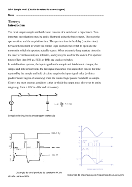
1290 Hammerwood Avenue
Sunnyvale, CA 94089
Phone (408) 745-0383 Fax (408) 745-0956
www.ondacorp.com
I. Methodology for Onda's Hydrophone Calibrations
Calibration is obtained by comparison techniques to reference hydrophones calibrated
by the National Physical Laboratory (NPL) in the UK. For calibration below 20 MHz, the
stepped single frequency comparison technique is used, and for calibration above 20
MHz, the harmonic comparison technique is employed. The procedures are as follows:
Stepped single frequency comparison technique:
1) The reference hydrophone is placed at the focus of a broadband source [1], which
is driven by a sinusoidal tone burst. The reference hydrophone is aligned by
maximizing the hydrophone signal with the source driven at the maximum end of
its frequency range (20 MHz for a 1-20 MHz calibration, 5 MHz for a 0.25-1 MHz
calibration). The voltage driving the source is then swept in across the frequency
range (i.e., 1 to 20 MHz, or 0.25 to 1 MHz). At each frequency, the output of the
reference hydrophone is measured and digitally filtered to separate the primary
frequency component from any harmonics that may be present in the signal. The
reference hydrophone has previously been calibrated by NPL, so that the voltage it
detects can be translated into a pressure value, hence calibrating the pressure
output of the source as a function of frequency, at the source’s focal position.
2) The reference hydrophone is then replaced by the hydrophone to be calibrated,
and re-aligned. The voltage driving the source is again swept across the same
frequency settings, and the output of the hydrophone at the fundamental of the
driving signal is determined and recorded. This voltage is then divided by the
pressure amplitude (measured in step 1) to determine the output of the
hydrophone in Volts per Pascal (V/Pa).
Harmonic comparison technique:
1) The reference hydrophone is placed at a position in the non-linear acoustic field
produced by a plane circular source transducer driven by a 2.25MHz sinusoidal
tone-burst signal. The position was chosen where many strong harmonics of the
fundamental frequency are generated in the distorted pressure waveform due to
non-linear propagation. Using a 50 MHz high-pass filter, the reference
hydrophone is aligned by maximizing the hydrophone’s high frequency
components in the plane at that position to an optimal orientation. The pressure
waveform at that position is recorded after the high-pass filter was removed. An
Onda_HydroCalMethod_20131018.doc
Page 1 of 6
FFT of the waveform is calculated, and the voltage amplitude at each harmonic is
determined. The reference hydrophone has previously been calibrated by NPL,
so that the voltage it detects can be translated into a pressure value, hence
calibrating the pressure output of the source at each harmonic.
2) The reference hydrophone is replaced by the hydrophone to be calibrated, which is
then aligned the same way at the same position as the reference hydrophone.
The pressure waveform is recorded with the absence of the high-pass filter. An
FFT of the pressure waveform is then calculated, and the voltage at each
harmonic is determined. This voltage is then divided by the pressure amplitude
(measured in step 1) to determine the output of the hydrophone in Volts per
Pascal (V/Pa).
II. Calibration Uncertainty
The uncertainties in the calibration are predominantly systematic in origin, the random
error is negligible in comparison. The dominant source of uncertainty is the uncertainty
in the calibration of the reference hydrophone (as provided by NPL). The other sources
of uncertainty are temperature variation (± 1 ºC, resulting in calibration variations of ±
1%) source stability (± 2%) digitizer error (± 2%) and positional repeatability (this effect
varies with frequency, from ± 2.5% at 1 Mhz to ± 5% at 20 MHz). The combined effect
of these error sources is calculated according to [2-3], with a coverage factor of k = 2 to
calculate the uncertainty with a 95% confidence level. This yields uncertainties that are
typically within ± 1.5 dB from 0.5 to 1 MHz, ± 1 dB from 1 to 15 MHz, ± 1.5 dB from 15
to 20 MHz, ± 2.2 dB from 20 to 40 MHz and ± 3 dB from 40 to 60 MHz.
Onda_HydroCalMethod_20131018.doc
Page 2 of 6
III. Important Considerations Regarding Electrical Loading
Conditions
HMA and HMB hydrophones are sold with a standard 1-20 MHz calibration into a
50-ohm load. HGL, HNP (formerly HNV), HNC (formerly HNZ), and HNR
hydrophones are modular—i.e., they allow the user to choose different amplifiers
or no amplifier at all. Because a hydrophone's sensitivity depends on the electrical
impedance of the detector or amplifier it is attached to, modular hydrophones are
sold with an open-circuit calibration, called formally the "End-of-cable Open Circuit
Sensitivity", or EOC sensitivity for short, and designated as M c ( f ) [4-5]. M c ( f )
is determined by measuring the sensitivity of the hydrophone with a laboratory
amplifier, and then subtracting the effect of that amplifier's gain, as well as that of
its finite (i.e., non-infinite load). Note that the HGL, HNP, and HNC hydrophones
may be connected directly to an amplifier without any cable, so the EOC sensitivity
is defined as the sensitivity that would be measured at the hydrophone's connector
into an infinite load.
Of course, actual hydrophone usage is made with the customer's choice of
amplifier and/or other form of detector. In such cases, the customer may calculate
the effect of the amplifier/detector configuration on the hydrophone sensitivity, by
mathematically combining hydrophone calibration data and amplifier data, as
described below:
Obtaining amplifier-loaded sensitivity from EOC data
The sensitivity of the hydrophone/preamp combination ( M L ( f ) ) can be
determined using the following formula [4]:


Re( Z A ) 2 + Im(Z A ) 2
M L ( f ) = G( f )M c ( f )
2
2 
{Re( Z A ) + Re( Z H )} + {Im( Z A ) + Im( Z H )} 
1/ 2
(1)
where
G ( f ) = amplifier gain (as a function of frequency)
Z A = input impedance of amplifier
Z H = impedance of hydrophone
Re( Z) indicates the real part of a complex number Z
Im( Z) indicates the imaginary part of a complex number Z
If the hydrophone and amplifier impedances are primarily capacitive (as is the case
with all Onda hydrophones and amplifiers), Eq. (1) can be approximated:
Onda_HydroCalMethod_20131018.doc
Page 3 of 6
CH
(2a)
CH + C A
where C A and C H and are the capacitance of the amplifier and hydrophone ,
respectively. C H is provided with the EOC calibration data shipped with each modular
hydrophone. Onda provides C A with the calibration sheets for all AH2010 and
AH2020 amplifiers, and can be purchased for an additional price for other Onda
amplifiers.
M L ( f ) = G( f ) M c ( f )
Note that in some cases, adaptors or short cables may be used between the
hydrophone connector and the amplifier. This additional connection length may have
an effect which can be approximated by a connection capacitance, designated C C ,
which can be accounted for by the following modification to Eq. (2):
M L ( f ) = G( f ) M c ( f )
CH
C H + CC + C A
(2b)
A common example of such a connector is the right angle SMA connector (Onda part number ARAMAF) which is used to connect an Onda HGL hydrophone to an AH2010 or AH2020 in a right-angle
configuration; C C = 1.6 pF for this case.
Note: Customers are advised to perform their own assessment of the accuracy
of Eqs. (2a-b) for their configuration. In particular, customers should be aware
that extension cables connecting the hydrophone to the preamplifier or detector
may not be accurately modeled as purely capacitive at higher frequencies; in
such cases, customers are advised to consider purchasing a separate calibration
which includes the use of their extension cables.
Onda_HydroCalMethod_20131018.doc
Page 4 of 6
IV. Other Common Calibration Units
M L ( f ) is in units of voltage divided by pressure and is typically expressed in V/Pa.
Alternatively, it can be expressed in units of dB re 1V/µPa using Eq. (3):
dBre 1V / µPa [ M L ( f )] = 20 * log10 [ M L ( f )] − 120
(3)
It is also common to express the calibration in terms of acoustic intensity. Strictly
speaking, a simple calibration factor exists only under conditions of a sinusoidal signal
and under the assumption that intensity is equal to the time-averaged value of the
pressure squared divided by the acoustic impedance of the medium. Under these
conditions the following relation applies:
I = V RMS / K
2
(4)
where I is the acoustic intensity, and V RMS is the root-mean-square voltage of the
sinusoidal signal. The calibration factor K is given by
K = z a [ M L ( f )]2
(5)
where z a is the acoustic impedance of the medium (1.5 MRayls for water). Because it
is common to express I in units of W/cm^2,
K {volts 2 cm 2 / Watt} = 1.5 x1010 [ M L ( f ){volts / Pa}] 2
for water
(6)
V. Examples
Example I. An HNV-0400 is supplied by Onda with an EOC calibration:
M c ( f ) = 50 nV/Pa at 5 MHz, and C H = 80 pF
We now wish to determine the sensitivity for this hydrophone connected to an AH-2010
preamplifier.
As determined from the datasheet for the AH-2010, the amplifier impedance is
capacitive with C A = 7 pF, and the gain is 20 dB ( G ( f ) = 10). Application of Eqs. (2a)
and 3 shows that M L (5MHz ) = 460 nV/Pa, or –246.7. dB re 1V/µPa. Application of Eq.
(6) yields K (5 MHz) = 3.17 x 10-3 V2 cm2/W.
Onda_HydroCalMethod_20131018.doc
Page 5 of 6
Example II. An HGL-0200 is supplied by Onda with an EOC calibration:
M c ( f ) = 45 nV/Pa at 5 MHz, and C H = 13 pF
We now wish to determine the sensitivity for this hydrophone connected to an AH-2010
preamplifier through an AR-AMAF connector:
As determined from the datasheet for the AH-2010, the amplifier impedance is
capacitive with C A = 7 pF, and the gain is 20 dB ( G ( f ) = 10). Application of Eqs. (2b)
and 3 shows that M L (5MHz ) = 271 nV/Pa, or –251.3dB re 1V/µPa. Application of Eq.
(6) yields K (5 MHz) = 1.10 x 10-3 V2 cm2/W.
References
[1] A. Selfridge and P.A. Lewin, “Wideband Spherically Focused PVDF Acoustic Source
for Calibration of Ultrasound Hydrophone Probes,” IEEE Trans. UFFC, 47(6) 13721376, 2000.
[2] R. C. Preston, D.R. Bacon, and R. A. Smith, “Calibration of Medical Ultrasound
Equipment: Procedures and Accuracy Assessment,” IEEE Transactions on Ultrasonics,
ferroelectrics, and Frequency Control, Vo. UFFC-25(2), pp. 110-121, 1988.
[3] M. C. Ziskin, “Measurement Uncertainty in Ultrasonic Exposimetry,” in Ultrasonic
Exposimetry, M.Ziskin and P. Lewin, eds. (CRC Press), Chapter 14, 1993.
[4] ALUM/NEMA: Acoustic Output Measurement Standard for Diagnostic Ultrasound
Equipment. American Institute of Ultrasound in Medicine, 14750 Sweitzer Lane, Suite
100, Laurel MD 20707-5906; National Electrical Manufacturers Association, 1300 North
17thStreet, Suite 1847, Rosslyn VA 22209.
[5] IEC 62127-2: Ultrasonics – Hydrophones – Part 2: Calibration for Ultrasonic Fields
Up to 40 MHz.
Onda_HydroCalMethod_20131018.doc
Page 6 of 6