Proceedings of COBEM 2009 Copyright © 2009 by ABCM 20th International Congress of Mechanical Engineering November 15-20, 2009, Gramado, RS, Brazil THE DETERMINATION OF THE TEMPERATURE DISTRIBUTION IN SOILS USING GITT (GENERALIZED INTEGRAL TRANSFORM TECHNIQUE) Manuella Andrade Pereira de Souza Silva, [email protected] Cristiane Kelly F. da Silva, [email protected] Universidade Federal da Paraíba – UFPB, Laboratório de Energia Solar, Castelo Branco, 58051-970, João Pessoa, Paraíba, Brasil Andréa Samara Santos de Oliveira, [email protected] Instituto Federal de Educação, Ciência e Tecnologia do Ceará, Campus Juazeiro do Norte, Av. Plácido Aderaldo Castelo, 1646, Planalto, 63040-000, Juazeiro do Norte, Ceará, Brasil Mirtes Aparecida da Conceição Silva, [email protected] Universidade Federal da Paraíba – UFPB, Laboratório de Energia Solar, Castelo Branco, 58051-970, João Pessoa, Paraíba, Brasil Zaqueu Ernesto da Silva, [email protected] Universidade Federal da Paraíba – UFPB, Laboratório de Energia Solar, Castelo Branco, 58051-970, João Pessoa, Paraíba, Brasil Antônio Carlos Cabral dos Santos, [email protected] Universidade Federal da Paraíba – UFPB, Laboratório de Energia Solar, Castelo Branco, 58051-970, João Pessoa, Paraíba, Brasil Abstract. The determination of the temperature distribution in soils is of interest for various knowledge fields, because its variation affects processes such as seed germination, plant growth and thermal behavior of buildings in direct contact. It is however a problem of many variables, due the temperature variation can be influenced by the characteristics and interactions between the elements of the system soil-vegetation-atmosphere. In this study, it was determined the temperature field considering only the heat transfer by conduction in homogeneous and onedimensional way. The function governing the temperature variation on the surface was considered as harmonic in time. For the solution of ordinary differential system, was used the GITT (Technique of Integral Transform), analytical-numerical method employed successfully in the past 20 years, mainly in the study of heat transfer. The basic idea is to transform the partial differential system in an ordinary differential system by expanding in eigefunctions. This system is solved numerically using subroutine established in mathematical literature available. Keywords: Soil Temperature, Temperature field, GITT 1. INTRODUCTION The climatic variations have been reason of the scientific community and all society’s concern. A great number of studies try to preview and/or describe climatic changes. In these studies, the energy balance at the surface is necessary, because it conditions the partition of the solar energy. Measurements of temperature at the soil become indispensable for us to feed the mathematical models allowing the climatic characterization of the area. The accuracy of these calculations depends on the knowledge of the materials thermal properties, specifically thermal diffusivity. Numerous examples of flaws can be mentioned and can be attributed to the bad quality of the information associated to the choice of the values of these properties. Several methods for temperature profile determination can be available numerical solutions as in Karam (2000), Mihalakakou (2002), analytical, in Gülser et al (2004), and also studies that compare the results gotten for these methods, Fuhrer (2000) and Chicota et al (2004). According to Musy et al (1991), the description of soil global thermal behavior, for instance, results from two types of phenomena: the energy exchanges with the exterior and a series of heat transfer processes. The intensity of these processes depends on the ground specific thermal properties. For Brady (1989), they are determinative factors in the energy partition that arrives in terrestrial surface. While the solar irradiation that arrives at the surface depends on climatic factors, the quantity of energy that penetrates in the ground depends on factors like soil color, declivity and vegetal covering at the considered area. In this work we will utilize the Generalized Integral Transform Technique (GITT) that is a well-known hybrid numerical–analytical approach that can efficiently handle diffusion and convection–diffusion partial differential formulations. It is based on expansions of the original potentials in terms of eigenfunctions and the solution is obtained through integral transformation in all but one of the independent variables, thus reducing the partial differential formulations to an ordinary differential system for the expansion coefficients, which can be then solved using numerical techniques or in some special cases, analytical procedures (Almeida et al., 2008). The Generalized Integral Transform Technique has quite recently appeared in the literature as an alternative to conventional discrete numerical methods, for various partial differential formulations in heat and fluid flow (Venezuela Proceedings of COBEM 2009 Copyright © 2009 by ABCM 20th International Congress of Mechanical Engineering November 15-20, 2009, Gramado, RS, Brazil et al., 2009, Naveira et al., 2007, Barros et al., 2006, Macêdo et al., 1999). Its hybrid numerical - analytical structure permits the automatic control of the global error in the simulation, which avoids the need for several computer program runs to inspect for the convergence on the final results, and therefore yields codes that automatically work towards user prescribed accuracy targets. A number of applications have been considered within the last few years dealing with environmental modeling, in relation to the hybrid approach here discussed. The present study aims to know the temperature profile determined from the solution using the Generalized Integral Transform and comparing this profile with that measured in the meteorological station in São João do Cariri-PB town. 2. PHYSICAL PROBLEM AND MATHEMATICAL MODELLING 2.1. Model assumptions The direct problem is solved to determine the temperature profile into the soil. The physical problem involves transient heat conduction and the temperature at the soil surface is expressed as a time harmonic function like in Horton et al (1983), Musy et al (1991) and Furher (2000). The following assumptions were adopted in order to simplify the model: The ground is represented by a semi-infinite plate of thickness 2L; Heat transfer is predominantly unidirectional; Shrinkage is negligible; The diffusion coefficient is constant and homogeneous during process. 2.2. Mathematical Modelling Based on the foregoing hypotheses, the equation describing heat transfer process is given as follows: T z , t 2T z , t at 0 < z < L t z 2 (1a) The initial and boundary conditions are listed below to complete the numerical formulation of the problem: Boundary conditions T 0, t T0 t Tmed Tsennt T z , t Tmed (1b) (1c) Initial condition T z ,0 Tini at 0 ≤ z ≤ L (1d) Where T (z, t) (°C) is temperature, z (m) the depth and t (s) the time. Assuming that apparent thermal diffusivity = k/C (m ² /s) is independent of temperature. The Eqs. (1) are given in dimensionless form by: Z , 2 Z , Z 2 0 < Z < 1, τ > 0 (2a) with boundary and initial conditions 0, sen Z = 0, τ > 0 (2b) Proceedings of COBEM 2009 Copyright © 2009 by ABCM 20th International Congress of Mechanical Engineering November 15-20, 2009, Gramado, RS, Brazil 1, 0 Z = 1, τ > 0 (2c) Z ,0 1 0 ≤ Z ≤ 1, τ = 0 (2d) where the dimensionless groups are: t ; L2 Z z ; L Z , T z , t Tmed Tini Tmed The objective now is to determine the process dimensionless temperature field. Mathematical model is solved here by applying the Generalized Integral Transform Technique (GITT) as described next. 2. METHOD OF SOLUTION FOR THE MATHEMATICAL MODEL The Generalized Integral Transform Technique (GITT) is a powerful hybrid numerical-analytical approach, which has been successfully used to obtain benchmark solutions for different classes of linear and non-linear diffusion/convection problems (Dantas et al., 2002). Such a technique, as applied to time dependent problems, includes the following basics steps: (i) Selection of an associated auxiliary eigenvalue problem, that retains the highest capacity of information of the original problem; (ii) Development of the appropriate transform/inverse formulae pair; (iii) Integral transformation of the original problem by substituting the inverse formula into non-transformable terms or by using the integral balance approach; (iv) Solving the resulting coupled system of ordinary differential equations in the time variable; (v) Appling the inverse formula to the transformed field in order to obtain the solution for the original problem. It can be seen that through dimensionless process was possible to obtain Z domain ranging from 0 to 1, but it was not possible to obtain homogeneous boundary conditions. Thus to solve the problem (2a-2d) by GITT it will be used solutions superposition, Diprima and Boyce (2002) with order to homogenize boundary condition (2b), which satisfy the requirements of the theory of the Sturm –Liouville problem, as follows: It will be proposed a main problem simpler version to find a filter. d 2 F (Z ) 0 ; F (0) sen( ) ; F (1) 0 dZ 2 (3a-c) Witch can be expressed by: F ( Z ) aZ b (3d) Replacing boundary conditions, we get: F ( Z ) sen( )1 Z (3e) F(Z) function will be used as a filter to homogenize boundary condition (2b). We define solutions superposition as: ( Z , ) F ( Z , ) F (Z ) (3f) Replacing Eq. (3f) in system equations (2), after some mathematical arrangements, the transformed problem to be solved is written by the following form: F Z , 2F Z , cos( )Z 1 Z 2 (4a) F 0, 0 (4b) Proceedings of COBEM 2009 Copyright © 2009 by ABCM 20th International Congress of Mechanical Engineering November 15-20, 2009, Gramado, RS, Brazil F 1, 0 (4c) F Z ,0 1 sen 1 Z (4d) Once obtained the transformed problem with homogeneous boundary conditions, Generalized Integral Transform Technique (GITT) can be applied (Ozisik, 1980). The first step is choosing the so-called auxiliary problem. If we consider the differential equation (4) with its boundary conditions, it can be expressed as (Ozisik, 1980): d 2 dZ 2 i2 i 0 (5a) i 0 0 (5b) i 1 0 (5c) Equations (5) represent a classical Sturm–Liouville problem. Its solution is obtained in the form of eigenfunctions and eigenvalues, respectively: i Z sin i Z i i i 1,2,3... The next step is to define the Transformed/Inverse pair 1 Ni Fi 1 0 iFdZ Transformed (6a) Inverse (6b) i Fi Ni i 1 F Z , where Fi is the transformed dependent variable and the norm Ni is given by: Ni 1 2 (6c) The normalized eigenfunctions are defined by: i Z i Z (6d) Ni Moreover, the eigenfunctions have the following orthogonality property: ~ ~ 0, i j i Z j Z dZ 1, i j At this point, the integral transformation can be applied. Eqs (4) is integrated using the operator (6e) Proceedings of COBEM 2009 Copyright © 2009 by ABCM 1 20th International Congress of Mechanical Engineering November 15-20, 2009, Gramado, RS, Brazil ~ i Z dZ 0 On the basis of the orthogonality property (6e), the Integral Transform (6a) and the Inverse Formula (6b), from Eq. (4) we get 1 d Fi i2 Fi cos i Z 1dZ d 0 (7a) The integral transform of the entry condition (Eq. (6a)) produces the following transformed initial condition: 1 Fi 0 1 sin 1 Z ~i dZ (7b) 0 Ordinary differential equations system presented in Eqs. (7) for the transformed potentials was solved in the Matlab. For computational purposes this system is truncated to a sufficiently large finite order, N, for the required convergence control. 3. RESULTS The problem considers the function that represents temperature profile with harmonic behavior. This comportment is showed in Fig. (1) for many different depths. The hybrid numerical-analytical solution of mass transfer problem was validated by experimental results given by the experiment carried in a meteorological station of UFPB in Solar Energy Laboratory at São João do Cariri-PB town (07°22’44” S; 36°32’00” W; and 465m above sea level) in southwest of Paraíba, from 06/05/2001 to 09/05/2001. The soil is covered with sparse vegetation (caatinga and pasture kind). The region is classified as semi-arid with less abundant rainfall concentrated between the months from February to April. The loamy soil is rocky type and the vegetation is sparse and gives the appearance of strips alternatively between the rocky soil and the bare soil, Paz (2002). Figure 1 – Harmonic behavior for temperature profile. Soil temperature was measured using temperature sensors (Campbell Scientific Inc., model 108) with precision of 0.3°C, operating over the range – 3 to 90°C, installed at the surface and in others three depths, 2, 5 and 15 cm. The measurements were taken with 20 minutes of interval by the data acquisition system CR23X of the Campbell Scientific Proceedings of COBEM 2009 Copyright © 2009 by ABCM 20th International Congress of Mechanical Engineering November 15-20, 2009, Gramado, RS, Brazil Incorporation, continuously connected to the battery of 12 V and 55 Ah, accompanied to a solar panel with potential of 50W. Data logger is programmed to control all the experiment and to unload the data to the microcomputer. 55 50 30 0 1 2 Teorical Experimental Residuals 3 4 20 10 40 35 -10 Residuals (ºC/Cº) Temperature (°C) Temperature (°C) 45 30 -20 25 20 -30 0 1 2 3 4 Figure 2 – Temperature profile at the surface. Observing the evolution of the temperature profile at 5 cm, the maximum temperature is 34.29°C that occurs at 19 p.m. in the first measurement day, the minimum was 30.86°C at 10 a.m. in the second measurement day. Taking visual analysis, we can verify that the temperature model-data was underestimated in the period except for the first day. The minimum values present less important residues although the model overestimates the real value. The residues have a maximum value of 0.86°C at 14 p.m. in the first day and the minimum was -0.001°C at 18 p.m. in the third day, the absolute average was 0.38°C. These values can show the coherence between model and experimental data. We can observe in the figures that the curves present the same behavior that the experimental data, harmonic. The model consistence is in the fact that thermal perturbation of solar irradiation which the ground is submitted presents similar behavior and mainly because model and experimental data presented a good approach with a standard deviation of 3.24°C that corresponds a relative standard deviation of 0.16% for 5 cm depth. For the measurements at the surface, the model coherence are not very good, there are many others factors that have a great importance like the days climatic conditions when the measurements had been made. We believe that de differences between the temperature model-prediction and field data can be eventually associate to the hypotheses made to arrive at the analytical solution, such as neglecting the evaporation, the dependence of the thermal diffusivity to the soil humidity, the soils homogeneity and the assumption that a complicated three-dimensional heat transfer process can be represented by an one-dimensional model. For obtain a better precision of the model, the data must be more studied and taken days with same climatic conditions (cloud presence, wind speed, rainfall). For modeling, we need to consider others accomplished heat transfer processes, irradiation and convection, that occur at surface and change boundary conditions. 4. REFERENCES Almeida, G. L., Pimentel, L. C. G. and Cotta, R. M., “Integral Transform Solutions for Atmospheric Pollutant Dispersion”, Environ Model Assess (2008) 13:53–65 DOI 10.1007/s10666-006-9072-4. Barros, F.P.J., Mills, W.B., Cotta, R.M., 2006, “Integral Transform Solution of a Two-Dimensional Model for Contaminant Dispersion in Rivers and Channels with Spatially Variable Coefficients”, Environmental Modelling & Software, Vol. 21, pp. 699-709. Brandy, N. C., 1989, Natureza e Propriedades dos Solos. 7 ed. Rio de Janeiro, Brasil, Livraria Freitas Bastos S/A. Boyce, W.E. e Diprima, r. C., 2002, “Equações Diferenciais Elementares e Problemas de Valor de Contorno”, L.T.C. Livros Técnicos e Científicos, Editora S.A., Rio de Janeiro. Dantas, L. B., Orlande, H. R. B. and Cotta, R. M., 2002, “Estimation of Dimensionless Parameters of Luikov’s System for Heat and Mass Transfer in Capillary Porous Media”, International Journal of Thermal Sciences, Vol. 41, pp. 217-227. Fuhrer, O., 2000, Inverse Heat Conduction In Soils – A New Approach Towards Recovering Soil Moisture fromTemperature Records. Diploma Thesis. Dept. Physics. ETH Zurich. Proceedings of COBEM 2009 Copyright © 2009 by ABCM 20th International Congress of Mechanical Engineering November 15-20, 2009, Gramado, RS, Brazil Gülser, C., Ekberli, M., 2004, “A Comparison of Estimated and Measured Diurnal Soil Temperature Through a Clay Soil Depth”, Journal of Applied Sciences, v. 4, pp. 418-423. Horton, R., WIERENGA, P.J., 1983a, “Estimating the Soil Heat Flux from Observations of Soils Temperature Near the Surface”, Soil Science Society of America Journal, v. 47, pp. 14-20. Horton, R., WIERENGA, P.J., NIELSEN, D. R., 1983b, “Evaluation of Methods for Determining the Apparent Thermal Diffusivity of Soil Near the Surface”, Soil Science Society of America Journal, v. 47, pp. 25-32. Karam, M. A., 2000, “A Thermal Wave Approach for Heat Transfer in a Nonuniform Soil”, Soil Science Society of America Journal, v. 64, pp. 1219-1225. Macêdo, E. N., Cotta, R. M. and Orlande, H. R. B., 1999, “Local-Instantaneous Filtering in the Integral Transform Solution of Nonlinear Diffusion Problems”, Computational Mechanics, Vol. 23, pp.524-532. Mihalakakou, G., 2002 “On Estimating Soil Surface Temperature Profiles”, Energy and Buildings, ELSEVIER, v. 34, pp. 251-259. Musy, A., Soutter, M., 1991, Physique du Sol. Collection Gerer l’Environnement. Paris. Presses Polytechiniques et Universitaires Romandes. Naveira, C.P., Lachi, M., Cotta, R.M. and Padet, J., 2007, “Integral Transform Solution of Transient Forced Convection in External Flow”, International Communications in Heat and Mass Transfer, Vol. 34, pp. 703–712. Ozisik, M.N., 1980. Heat Conduction,. John Wiley & Sons, New York, 704 pp. Venezuela, A. L., Pérez-Guerrero, J. S. and Fontes, S.R., 2009, “Hybrid Modeling of Convective Laminar Flow in a Permeable Tube Associated with the Cross-Flow Process”, Communications in Nonlinear Science and Numerical Simulation, Vol. 14, pp. 795–810. 5. RESPONSIBILITY NOTICE The authors are the only responsible for the printed material included in this paper.
Download