Week 4
Market Failure due to ‘Moral Hazard’
The Principal-Agent Problem
Principal-Agent Issues
Adverse selection arises because one side of the market cannot observe the
quality of the product or the customer on the other side: consequently, it is
sometimes referred to as a hidden information problem. A related issue is the
fact that the actions of a person in transaction may not be observable by the
other party (parties) to the transaction. This may then lead the party, whose
action cannot be observed, to be ‘negligent’, or to not take ‘due care’, in
fulfilling his duties with respect to the transaction. This is referred to as moral
hazard or a hidden action problem and it underpins issues of principal-agent
interaction.
Hidden Action: Efficiency Wages
1. Workers employed in modern industry have some control over their own
productivity. They can choose their ‘effort’ and they put in more effort
when they are motivated to do so.
2. In the absence of motivation, workers will shirk. Even if they are caught
shirking and fired, they can easily find another job if the wage is market
clearing so that there is no unemployment.
3. One way for employers to provide motivation is to pay more than other
employers; another is to fire those who are shirking. But firing will only be
effective if it is difficult to find another job.
4. Workers provide effort because to be found shirking and fired is costly.
Costly because of the loss of ‘higher than market’ wages; costly because
with a non-zero unemployment rate, it is difficult to find another job.
5. Workers are motivated, therefore, by the carrot of higher wages and by the
stick of dismissal (and the difficulty of finding another job). For the stick to
work, unemployment is necessary.
If the effort that the worker puts in is not observable by the firm then it has two
alternatives: the firm can motivate the worker by providing a wage higher than
the market clearing wage; the firm can monitor the effort of the worker and
threaten to fire those whose effort is unacceptably low. The higher the current
rate of unemployment, and the higher the wage paid over the market wage,
the more effective will be the threat of dismissal (Yellen, 1984).
Source: Pindyck and Rubenfeld (2001), p. 618
Labour supply
No Shirking Constraint
wE
*
w
A
Labour demand
LA
LE
*
L
Figure 12:
Efficiency Wages
In Figure 12, the market clearing wage w* equates labour demand with labour
supply. However, when workers are paid w*, they have an incentive to ‘shirk’:
even if they are detected and fired, they can find a job with another employer
for the same wage because, by definition, there is no unemployment. So the
firm has to offer an ‘efficiency wage’ wE>w* so that there is ‘no shirking’. This
efficiency wage is shown by the ‘no-shirking constraint’ curve in Figure 12.
This curve shows, for each level of labour usage, the minimum wage that
workers need to be paid so that they do not shirk. At the point A, labour
usage is LA and unemployment is L*-LA: workers only need to be paid the
competitive wage, w*, to induce them not to shirk; as labour usage rises, so
that the unemployment rate falls, the efficiency wage rises above the
competitive wage. The equilibrium efficiency wage – which all firms in the
industry pay – is wE, given by the intersection of the labour demand and the
‘no shirking’ curve. Unemployment is L*-LE and workers do not shirk at wE
because the positive amount of unemployment at wE means they would not
be certain of finding another job if they were fired for shirking.
Efficiency Wages: Formal Analysis
The production function of the firm is: y = f ( L, e), ∂f / ∂L > 0, ∂f / ∂e > 0 where e
is effort, e = g ( w), de / dw > 0 . The firm’s maximisation problem is:
Max
N π = pf ( L, e) − wL
w, L
(1)
st : e = e( w), w ≥ w
Then the first order conditions for a maximum are:
∂f ( L, e)
p
−w=0
∂L
∂f ( L, e) de
p
−L=0
∂e dw
(2)
Combining the two equations in (2):
fL
( L / y) f L
w
we′( w)
= ⇒
=
f e e′( w) L
f e (e( w) / y )
e( w)
(3)
The RHS of equation (3) is the elasticity of effort with respect to wages: if
ε=
we′( w)
, then, if wages go up by 1%, effort will go up by ε % .
e( w)
The LHS of equation (3) may be interpreted as the ratio of the elasticity of
output with respect to employment to the elasticity of output with respect to
effort .
Now suppose that y = f ( Le) ⇒ f L = f ′( Le)e and f e = f ′( Le) L so that equation
(3) becomes:
we′( w)
=1
e( w)
(4)
Equation (4) represents the key efficiency wage theorem: the wage is set so
as to elicit 10% more effort for 10% higher wages and is independent of
product and labour market conditions.
Full Information
The analysis1 first assumes that there is no hidden action problem: the action
of the agent can be observed by the principal. A firm is hiring a worker to do
a job. The output of the worker, y, depends amount of ‘effort’, x, that the
worker puts in: y=y(x); the payment to the worker, s, depends upon the output
1
Varian (2003), p. 679.
produced: s=s(y). The firm would like to choose the payment function, s(y),
so as to maximise its surplus: y – s(y).
However, the worker finds effort to be costly and c=c(x) denotes the cost of
effort. The utility of a worker who chooses effort x is: s(y(x)) – c(x). If u is
his ‘reservation’ utility level, then the participation constraint is:
s ( y ( x )) − c ( x ) ≥ u
(5)
Given this constraint, the firm wants the worker to choose x so as to maximise
surplus:
Max y ( x) − s ( y ( x )) st s ( y ( x )) − c( x) = u
(6)
x
It is assumed that the firm can perfectly observe the effort of the worker so
there is no asymmetry of information.
Substituting the constraint into the objective function in equation (13) yields:
Max y ( x) − [c ( x ) + u ]
(7)
x
and the first order conditions for this are:
y′( x) = c′( x)
(8)
or the marginal product from extra effort = marginal cost of extra effort.
Suppose x* is the optimal level of effort which the firm wants to extract from
the worker. Then the incentive scheme s(y) must be such that x* gives the
worker the highest level of utility:
s ( y ( x* )) − c ( x* ) ≥ s ( y ( x )) − c ( x) ∀x
(9)
The constraint embodied in equation (16) is the incentive compatibility
constraint.
So, the incentive scheme s(y) must satisfy the participation constraint
(equation (12)) and the incentive compatibility constraint (equation (16)).
Rent The worker could pay a fixed amount, call it ‘rent’ (R), to the firm and
keep the remainder. Then the payment scheme is:
s ( y ( x )) = y ( x ) − R
(10)
If the worker chooses effort so as to maximises his utility, s(y(x))-c(x), then
under ‘rent’ his problem is:
Max y ( x) − c( x) − R
x
(11)
and the first order conditions for this are: y′( x) = c′( x) so that the worker
supplies the optimal level of effort x*. The optimal rent, R*, is that which is
exactly high enough (equation (12)) to induce the worker to participate:
R* = y ( x ) − c( x) − u
(12)
Wages Now the worker is paid a wage, w, per unit of effort plus a lump sum,
K, so that the payment scheme is:
s ( x) = wx + K
(13)
The worker then chooses effort so as to maximise:
wx + K − c( x)
(14)
and the first order conditions for this are w = c′( x) . So, if the wage paid is
equal to the worker’s marginal product, he will choose the optimal level of
effort given by equation (15). The payment K is chosen so that:
K = u + c( x) − c′( x) x .
Take-it-or-leave-it Under this scheme, the worker receives a payment K* for
an effort level of x*, nothing otherwise, where K* satisfies the participation
constraint: K * = u + c( x* ) . If x≠x*, then he receives utility –c(x), but if x=x*,
utility is u : hence x=x*, is the optimal choice.
Sharecropping Under sharecropping, the worker and the firm each receive a
fixed share of output (respectively, α and 1-α). Suppose the worker receives:
s ( x) = α y ( x ) + K , where K is a fixed payment and α<1. Then the worker
chooses x to maximise:
α y ( x) + K − c( x)
(15)
and, at an optimum: α y′( x) = c′( x) . This violates the condition for optimum
effort of equation (15): y′( x) = c′( x) .
Under all the schemes, the worker chooses x so as to maximising his utility:
s(y(x))-c(x). This implies that he chooses his effort by equating the marginal
benefit of effort with its cost. The firm wants him to choose his effort so as to
equate the marginal product of effort with its cost. This can be achieved if the
payment scheme provides a marginal benefit to the worker which is equal to
his marginal product. All such schemes are incentive-compatible (Rent;
Wages; Take-it-or-leave-it) and, therefore, efficient; any scheme that does not
provide a marginal benefit equal to marginal product is not incentivecompatible and, therefore, inefficient.
Incentive and Participation Constraints
A landowner produces rice using labour and capital. The owner wants to
maximise rice production but has to rely on a worker whose effort will
influence the output of rice and hence affect profits. In addition to the effort of
the worker, rice production is affected by rainfall.
Poor Rainfall (p=0.5)
Good Rainfall (p=0.5)
Low effort (e=0)
$10,000
$20,000
High effort (e=1)
$20,000
$40,000
Cost of effort, c0 with low effort and c1 with low effort. The payment scheme
links wages, w to output: w=f(y).
Suppose the owners offer a fixed wage payment: w*. Since the worker does
not share in any of the gains from effort: e=0 and expected output ye=
$15,000
Suppose the payment scheme is:
If y=$10,000 or $20,000 w=w0; If y=$40,000 w=w1
So high effort generates an expected payment of: w00.5+ w10.5= (w0+ w1)/2 –
c1
Low effort generates an expected payment of: w0-c0
So worker has an incentive to put in high effort provided: (w0+ w1)/2 –c1>w0-c0
Worker has an incentive to participate provided w0>c0
Owner is better off since expected revenue is now $30,000 instead of $15,000
Now consider the following scheme: when y>y* w2=y-y*; otherwise w=w1.
Under what conditions will this satisfy the incentive constraint?
Now go back to the example of the previous week. Putting in high effort in
work is to accept a gamble with ER=(w0+ w1)/2 –c1. On the other hand, to
put in low effort is to reject the gamble and so receive w0-c0 with certainty.
The worker would decide whether to accept or reject the gamble by
comparing: u(w0-c0) with EU=[u(w1-c1)+u(w0-c1)]/2
If the worker is risk averse and (w0+ w1)/2 –c1= w0-c0 (that is, it is a fair
gamble) he will reject the gamble and not put in the effort.
So to induce him to accept the gamble, ER=(w0+ w1)/2 –c1>w0-c0. This
means that w1, the payoff in the good situation must be sufficiently high (we
assume w0 is a subsistence/minimum wage that can’t be lowered).
How high w1 needs to be depends on worker’s aversion to risk.
Baixar