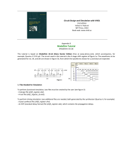
sid.inpe.br/mtc-m21b/2014/09.24.16.28-TDI
THE ROLE OF COMPUTATIONAL STEERING IN
SPACE ENGINEERING ACTIVITIES ASSISTED BY
MODELLING AND SIMULATION
Leandro Toss Hoffmann
Doctorate Thesis of the Graduate Course in Space Engineering and Technology/Space Systems
of Management and Engineering,
guided by Dr. Leonel Fernando
Perondi, approved in november 27,
2014.
URL of the original document:
<http://urlib.net/8JMKD3MGP5W34M/3H56LQH>
INPE
São José dos Campos
2014
PUBLISHED BY:
Instituto Nacional de Pesquisas Espaciais - INPE
Gabinete do Diretor (GB)
Serviço de Informação e Documentação (SID)
Caixa Postal 515 - CEP 12.245-970
São José dos Campos - SP - Brasil
Tel.:(012) 3208-6923/6921
Fax: (012) 3208-6919
E-mail: [email protected]
COMMISSION OF BOARD OF PUBLISHING AND PRESERVATION
OF INPE INTELLECTUAL PRODUCTION (DE/DIR-544):
Chairperson:
Marciana Leite Ribeiro - Serviço de Informação e Documentação (SID)
Members:
Dr. Gerald Jean Francis Banon - Coordenação Observação da Terra (OBT)
Dr. Amauri Silva Montes - Coordenação Engenharia e Tecnologia Espaciais (ETE)
Dr. André de Castro Milone - Coordenação Ciências Espaciais e Atmosféricas
(CEA)
Dr. Joaquim José Barroso de Castro - Centro de Tecnologias Espaciais (CTE)
Dr. Manoel Alonso Gan - Centro de Previsão de Tempo e Estudos Climáticos
(CPT)
Dra Maria do Carmo de Andrade Nono - Conselho de Pós-Graduação
Dr. Plínio Carlos Alvalá - Centro de Ciência do Sistema Terrestre (CST)
DIGITAL LIBRARY:
Dr. Gerald Jean Francis Banon - Coordenação de Observação da Terra (OBT)
Clayton Martins Pereira - Serviço de Informação e Documentação (SID)
DOCUMENT REVIEW:
Simone Angélica Del Ducca Barbedo - Serviço de Informação e Documentação
(SID)
Yolanda Ribeiro da Silva Souza - Serviço de Informação e Documentação (SID)
ELECTRONIC EDITING:
Marcelo de Castro Pazos - Serviço de Informação e Documentação (SID)
André Luis Dias Fernandes - Serviço de Informação e Documentação (SID)
sid.inpe.br/mtc-m21b/2014/09.24.16.28-TDI
THE ROLE OF COMPUTATIONAL STEERING IN
SPACE ENGINEERING ACTIVITIES ASSISTED BY
MODELLING AND SIMULATION
Leandro Toss Hoffmann
Doctorate Thesis of the Graduate Course in Space Engineering and Technology/Space Systems
of Management and Engineering,
guided by Dr. Leonel Fernando
Perondi, approved in november 27,
2014.
URL of the original document:
<http://urlib.net/8JMKD3MGP5W34M/3H56LQH>
INPE
São José dos Campos
2014
Cataloging in Publication Data
Hoffmann, Leandro Toss.
H675r
The role of computational steering in space engineering activities assisted by modelling and simulation / Leandro Toss Hoffmann. – São José dos Campos : INPE, 2014.
xxx + 239 p. ; (sid.inpe.br/mtc-m21b/2014/09.24.16.28-TDI)
Thesis (Doctorate in Space Engineering and Technology/Space
Systems of Management and Engineering) – Instituto Nacional de
Pesquisas Espaciais, São José dos Campos, 2014.
Guiding : Dr. Leonel Fernando Perondi.
1. Computerized simulation 2. Space systems engineering
3. Steering 4. Human-computer interface. 5. Software reuse.
I.Title.
CDU 629.78:004
Esta obra foi licenciada sob uma Licença Creative Commons Atribuição 3.0 Não Adaptada.
This work is licensed under a Creative Commons Attribution 3.0 Unported License.
ii
“ ‘en avant’ . . . ce doit être la devise de l’humanite!”
“ ‘avante’... este deve ser o lema da humanidade!”
Jules Verne, 1881
v
AGRADECIMENTOS
Ao longo dos últimos anos, diversas pessoas e instituições contribuíram de maneira
fundamental para que os resultados desta pesquisa fossem alcançados.
Inicialmente, gostaria de agradecer profundamente ao professor Leonel Fernando
Perondi, Ph.D., por aceitar a orientação deste trabalho e guiar sua evolução com
sabedoria e incansáveis aulas, não somente em temas da área espacial, mas também
sobre o nosso papel no desenvolvimento de uma sociedade mais igualitária.
Agradeço também aos membros da banca pela disponibilidade e dedicação em
participar da defesa, contribuindo com valiosas contribuições para o aperfeiçoamento
desta pesquisa.
Aos diversos docentes do curso de pós-graduação em Engenharia e Tecnologia
Espaciais ofereço minha gratidão e respeito pelos conhecimentos transmitidos. Em
especial à professora Dra. Ana Maria Ambrosio da qual recebi os primeiros conceitos
de simuladores de satélites.
Muito tenho em agradecer aos diversos colegas do Instituto Nacional de Pesquisas
Espaciais, pela troca de experiências e por contribuições que, mesmo de maneira
informal, foram decisivas no direcionamento do trabalho. Em particular, cito o meu
amigo e colega Mario Celso Padovan de Almeida que me ensinou diversos princípios
fundamentais de engenharia espacial.
Aos colegas da Divisão de Desenvolvimento de Sistemas de Solo, na pessoa de Rubens
Gatto, pela disponibilidade e apoio no progresso deste trabalho. Em especial à
futura doutora Denise Rotondi de Azevedo com a qual realizei diversos estudos
aprofundados no tema de simulação de satélites. Também ao amigo Joaquim Pedro
Barreto que realizou a organização do código fonte das interfaces do padrão SMP2.
À equipe de desenvolvimento do sistema de controle e atitude da Plataforma
Multi-Missão Brasileira, de maneira muito especial aos professores Dr. Roberto
Vieira da Fonseca Lopes e Dr. Ijar Milagre da Fonseca, com os quais tive o privilégio
de trabalhar e absorver uma pequena parcela de suas experiências.
Aos bolsistas do projeto de capacitação em software de controle de atitude de
satélites para a eletrônica de suporte de solo, apoiado pelo Conselho Nacional de
Desenvolvimento Científico e Tecnológico (CNPq), pela contribuição na modelagem
e verificação de componentes de simulação utilizados neste trabalho.
vii
Ao grupo de subsistema térmico do INPE, na pessoa do Dr. Douglas Silva e ao
professor Dr. Fabiano Luis de Sousa pelo suporte no uso da ferramenta Sinda/Fluint
e na modelagem dos cenários de térmica.
À equipe do projeto de Sistemas Inerciais para Aplicações Aeroespacial (SIA), na
pessoa do Prof. Dr. Waldemar de Castro Leite Filho por apoiar o desenvolvimento
do protótipo utilizado neste trabalho e ao Prof. Dr. Valdemir Carrara pelos
conhecimentos transmitidos.
Aproveito esta oportunidade para expressar minha gratidão e sincero apreço aos
colegas do Centro Europeu de Investigação e Tecnologia Espaciais (European
Space Research and Technology Centre – ESTEC), da Agência Espacial Europeia,
por propiciar o aprofundamento dos conhecimentos práticos em técnicas de
infraestruturas de simulação e validação de computadores de bordo. Em particular
ao Eng. Joachim Fuchs por viabilizar os estágios e aos líderes Eng. Kjeld Hjortnaes
e Eng. Robert Blommestijn, juntamente com os demais colegas de departamento,
por me receberem em suas instalações,. Em especial ao Eng. Quirien Wijnands que
conduziu minhas atividades com grande mestria e garantiu que minhas metas de
aprendizado fossem atingidas 1 .
Ao meu irmão Eng. Cleber Toss Hoffmann pelo imenso companheirismo e pelo apoio
técnico no desenvolvimento do estudo de caso com hardware na malha.
Finalmente, mas não menos importante, à minha esposa Laura, filha Gisele e mãe
Goret que me acompanharam nesta trajetória, provendo o suporte emocional e
incentivo para a conclusão deste projeto.
1
ACKNOWLEDGEMENTS: I take this opportunity to express my gratitude and sincere
appreciation to the colleagues from the European Space Research and Technology Centre
(ESTEC) of the European Space Agency, for making possible the development of my practical
skills in simulation infrastructures and on-board computer validation techniques. Particularly to
Mr. Joachim Fuchs for enabling the internships and to Mr. Kjeld Hjortnaes and Mr. Robert
Blommestijn, together with other department colleagues, to welcome me into their facilities. Special
thanks to Mr. Quirien Wijnands for guiding my activities with great mastery and for ensuring that
my learning goals could be achieved.
viii
ABSTRACT
Nowadays, computational simulation has a fundamental role on supporting
engineering activities across the life cycle of a space mission. As a consequence,
the pursuit for leaner processes and flexible tools has been the focus of numerous
investigations in the system engineering and simulation fields. In this direction, the
current work presents a novel approach for designing and conducting scenario of
spacecraft simulation, envisaging the improvement of space engineering practices by
employing computational steering methods. In the context of a scientific application,
steering is a technique to enhance the level of user interaction in a computational
system in order to allow a specialist to actively guide the course a simulation,
by on-line changing model parameters and visually monitoring the effects on the
scenario. In order to achieve such level of interactivity, in this work, an advanced
simulation facility is proposed to combine state of art concepts on satellite simulation
and the most relevant features of computational steering. The benefits of applying
these concepts in the development of space systems are demonstrated in case studies
inspired in real life problems, such as the verification and validation of a piece of
flight software, commonly adopted to determine the direction of Sun on-board the
spacecraft. The results have shown that the improvement of user interactivity in the
spacecraft simulation is a promising approach to deal with geometrically complex
scenarios and problems with high number of parameters, thereby contributing to
streamline manifold space engineering processes.
ix
O PAPEL DO ESTERÇAMENTO COMPUTACIONAL NAS
ATIVIDADES DE ENGENHARIA ESPACIAL ASSISTIDAS POR
MODELAGEM E SIMULAÇÃO DE SISTEMAS
RESUMO
Hoje em dia, a simulação computacional tem um papel fundamental no apoio às
atividades de engenharia ao longo de todo o ciclo de vida de uma missão espacial.
Como consequência, a busca por processos mais enxutos e ferramentas flexíveis
tem sido o foco de inúmeras investigações nas áreas de engenharia de sistemas e
simulação. Neste sentido, o presente trabalho apresenta uma nova abordagem para
a concepção e condução de cenários de simulação de plataformas orbitais, visando
à melhoria das práticas de engenharia espaciais por meio do emprego de métodos
de esterçamento computacional. No contexto de aplicações científicas, esterçamento
é uma técnica para melhorar o nível de interação do usuário em um sistema
computacional de modo a permitir que um especialista possa guiar ativamente o
curso de uma simulação, alterando parâmetros de modelos em tempo de execução
e monitorando visualmente os efeitos no cenário. De maneira a atingir tal nível de
interatividade, neste trabalho um ambiente avançado de simulação é proposto para
combinar conceitos do estado da arte em simulação de satélite e as características
mais relevantes de esterçamento computacional. Os benefícios da aplicação desses
conceitos no desenvolvimento de sistemas espaciais são demonstrados em estudo
de casos inpirados em problemas reais, tais como a verificação e validação de um
artefato de software de voo, comumente empregado na determinação da direção
do Sol a bordo da espaçonave. Os resultados mostraram que a melhoria da
interatividade do usuário na simulação de satélites é uma abordagem promissora
para se lidar com cenários geometricamente complexos e problemas com elevado
número de parâmetros, contribuindo assim para tornar mais ágeis diversos processos
de engenharia espacial.
xi
LIST OF FIGURES
Page
1.1
1.2
1.3
1.4
Logical workflow representing the strategy for developing this thesis. . . 3
Typical life cycle adopted in space engineering projects. . . . . . . . . . . 6
The adoption of V-Model supported by Modelling and Simulation. . . . . 8
Positioning of the contribution of thesis within the related fields of study. 11
2.1
2.2
2.3
2.4
Historical simulation usage in ESA along the spacecraft project’s life cycle.
Generic attitude control system and simulated elements. . . . . . . . . .
Overall architecture of an avionics testing equipment. . . . . . . . . . . .
Space engineering activities supported by simulation infrastructures
along project’s life cycle. . . . . . . . . . . . . . . . . . . . . . . . . . . .
High level overview of SMP2 standard. . . . . . . . . . . . . . . . . . . .
2.5
3.1
3.2
3.3
3.4
3.5
4.1
4.2
4.3
5.1
5.2
5.3
5.4
5.5
Types of visualization techniques with different levels of user interaction
in scientific simulations. . . . . . . . . . . . . . . . . . . . . . . . . . .
A textual interface in which the Bash command processor is used to
operate a computational system. . . . . . . . . . . . . . . . . . . . . .
Example of a GUI application containing windows, menus, buttons and
other graphical elements. . . . . . . . . . . . . . . . . . . . . . . . . . .
A 3D widget to graphically manipulate orbital parameters. . . . . . . .
Example of a virtual reality environment. . . . . . . . . . . . . . . . . .
17
20
21
24
26
. 31
. 36
. 37
. 39
. 40
Timeline of sequential steps in a simulation session conduced by a script
to perform the verification of three hypotheses. . . . . . . . . . . . . . . 54
Timeline of action in a simulation session conduced with computational
steering to perform the verification of three hypotheses. . . . . . . . . . . 55
Timeline of step required to verify three hypotheses with adjustments of
scenario script. . . . . . . . . . . . . . . . . . . . . . . . . . . . . . . . . 56
Overall architecture of computational steering facility. . . . . . . . . . .
Simulation infrastructure architecture. . . . . . . . . . . . . . . . . . .
SimuBox’s Simulation Development Kit elements. . . . . . . . . . . . .
Codification of MyModel class supported by sbLib. . . . . . . . . . . . .
Architecture detailed with components that enable computational
steering in the simulation infrastructure: steerable fields mechanism,
widget back-end, adapter component and catalogue, and remote widget
back-end. . . . . . . . . . . . . . . . . . . . . . . . . . . . . . . . . . .
xiii
.
.
.
.
70
71
72
73
. 75
5.6
5.7
5.8
5.9
5.10
5.11
5.12
5.13
5.14
5.15
5.16
5.17
5.18
5.19
6.1
6.2
6.3
6.4
6.5
Message invocation sequence originated by a remote adapter over TCP/IP.
Logical sequence of activities performed by the steering adapter. . . . . .
Class diagram of steering layer showing relationship between widgets,
adapters and steerable fields. . . . . . . . . . . . . . . . . . . . . . . . .
Differences on transferring data from output to input field when their
values are forced. . . . . . . . . . . . . . . . . . . . . . . . . . . . . . . .
Class diagram with steering mechanism for forcing model parameters. . .
Meta-model adopted to describe steering adapters. . . . . . . . . . . . .
Model tree loaded from the simulation configuration and their field values
visualization during execution. . . . . . . . . . . . . . . . . . . . . . . . .
Event viewer window used to display messages logged from simulator
kernel and model. . . . . . . . . . . . . . . . . . . . . . . . . . . . . . . .
History tree dialog used to load a playback session. The selected scenario
is composed of fragments of history data up to a root node. (A) is a root
node in the history tree that have been branched to (B) and the latter
to (C). . . . . . . . . . . . . . . . . . . . . . . . . . . . . . . . . . . . . .
Playback control panel: (A) execution control; (B) simulation horizon
slider; (C) acceleration factor slider and edit fields; (D) scenario branch
generation. . . . . . . . . . . . . . . . . . . . . . . . . . . . . . . . . . .
Main window of GUI for monitoring the simulation, provided by a client
application. . . . . . . . . . . . . . . . . . . . . . . . . . . . . . . . . . .
3D view of spacecraft’s orbiting Earth: (A) umbral shadow cone; (B)
orbit tube; (C) Sun direction w.r.t. Earth’s centre; (D) spacecraft position.
3D view of spacecraft’s attitude: (A) Reference frame; (B) Body frame;
(C) Sun direction w.r.t. body’s centre. . . . . . . . . . . . . . . . . . . .
Screenshot of generic steering application with a 3D vector widget
connected to the Sun position field. . . . . . . . . . . . . . . . . . . . . .
Simulation assembly for the spacecraft dynamics and environmental
models. . . . . . . . . . . . . . . . . . . . . . . . . . . . . . . . . . . .
Simulation assembly defining connections between the environmental
models and sensors. . . . . . . . . . . . . . . . . . . . . . . . . . . . . .
Simulation assembly defining the composition of eight Coarse Solar
Sensor models, their fixed shadow masks and the connections with the
environmental and power models. . . . . . . . . . . . . . . . . . . . . .
Simulation assembly of power subsystem models and their connections
with OBC and environmental models. . . . . . . . . . . . . . . . . . . .
Assembly for the software configuration of the on-board components,
which are implemented as simulation models. . . . . . . . . . . . . . .
xiv
75
76
77
78
79
80
81
82
83
83
84
85
86
87
. 94
. 96
. 97
. 98
. 99
6.6
6.7
6.8
6.9
6.10
6.11
6.12
6.13
6.14
6.15
6.16
6.17
6.18
6.19
Assembly for the hardware-in-the-loop configuration, in which the
on-board components are embedded in an independent platform and all
the communicate with the simulation is handled by the ObcIF model. .
Physical architecture of simulation facility. . . . . . . . . . . . . . . . .
Enhanced 3D visualization system for supporting the steering
interactions in the Sun Determination case studies. 1-8: coarse solar
sensors; A: solar panels; B: normal of solar panels; C: Sun vector (BF);
D: sensor’s plane; E: shadow mask applied to the sensor; F: Sun vector
as seen from the sensor. . . . . . . . . . . . . . . . . . . . . . . . . . .
Sequence of actions for Sun position and solar panel orientation steering
and corresponding simulation results. . . . . . . . . . . . . . . . . . . .
Assessment of SAG’s shadow effect on the Coarse Solar Sensors. The
visual output provides a tacit feedback on the model’s correctness. When
orienting the −Y panel at 45o it is clear that Sun is being blocked for
CSS6 (arrows in a,b) and illuminating it when panel is oriented at 315o
(arrows in c,d). . . . . . . . . . . . . . . . . . . . . . . . . . . . . . . .
A sequence of interactions performed to modify the solar panel’s
geometry and investigate its effects on the shadow model. A direct image
manipulation mechanism allows the engineer to steer the simulation
parameters with the same 3D visualisation interface. . . . . . . . . . .
Assessing the commanded solar panel’s orientation as function of Sun
vector. . . . . . . . . . . . . . . . . . . . . . . . . . . . . . . . . . . . .
The usage of special widget for steering the Sun vector with well-defined
irradiance levels (between 1310 and 1405 W/m2 ). . . . . . . . . . . . .
Fault tree diagram of the attitude determination module. . . . . . . . .
Sub-assembly of the on-board elements containing the FDIR module and
a stub for the attitude determination component. . . . . . . . . . . . .
Timeline of testing activities planned in the scenario. . . . . . . . . . .
GUI of the computational steering facility used in the on-board software
verification scenario: (A) 3D visualisation system; (B) infrastructure;
(C) Widget for steering the orbital parameters; (D) Simulation monitor
computing the Sun determination error; and widgets to steer the (E)
SAG’s orientation; (F) body rates; (G) attitude quaternion; and (H)
Sun’s position. . . . . . . . . . . . . . . . . . . . . . . . . . . . . . . .
Timeline of testing activities performed in the scenario. . . . . . . . . .
Evolution of error events and fault detection flags in the FDIR along the
simulation horizon. . . . . . . . . . . . . . . . . . . . . . . . . . . . . .
xv
. 100
. 101
. 103
. 106
. 108
. 109
. 111
. 113
. 115
. 116
. 116
. 119
. 120
. 121
6.20 Evolution of control variables used in addition to the visual feedback
during the scenario execution. . . . . . . . . . . . . . . . . . . . . . . . . 122
6.21 Orbit and corresponding nadir pointing attitudes in the beginning of the
scenario and after the 1st and 2nd user interventions. . . . . . . . . . . . 124
6.22 Dynamic dependencies of simulation models for the Sun Determination
scenario and some possible user interactions. . . . . . . . . . . . . . . . . 127
6.23 Investigation of a recurrent effect on Sun Determination error when a
given Sun/SAG geometry exists and an Earth’s Albedo vector is injected
on the solar sensors. . . . . . . . . . . . . . . . . . . . . . . . . . . . . . 129
6.24 Scheme of target geometrical configuration for investigation of control
behaviour when manoeuvring from Nadir to Sun pointing. . . . . . . . . 131
6.25 Orbital parameters steering for searching to a simulation state to comply
with the geometrical configuration from the Figure 6.24. . . . . . . . . . 133
6.26 Evolution of Sun pointing manoeuvre representing 16 seconds of
simulation time. . . . . . . . . . . . . . . . . . . . . . . . . . . . . . . . . 135
6.27 Behaviour of Sun pointing manoeuvre a (SAG Orient.=180o ;
Torque=unlimited; CSS Min. Elev.=0o ; none CSS Failures). . . . . . . . 136
6.28 Behaviour of Sun pointing manoeuvre b (SAG Orient.=90o ;
Torque=unlimited; CSS Min. Elev.=0o ; none CSS Failures). . . . . . . . 137
6.29 Sun determination error when a failure is injected in solar sensor +X+Y-Z.137
6.30 Behaviour of Sun pointing manoeuvre c (SAG Orient.=180o ;
Torque=unlimited; CSS Min. Elev.=0o ; Failure applied to +X+Y-Z
sensor). . . . . . . . . . . . . . . . . . . . . . . . . . . . . . . . . . . . . 138
6.31 Behaviour of Sun pointing manoeuvre d (SAG Orient.=180o ;
Torque=limited to 5Nm; CSS Min. Elev.=0o ; Failure applied to +X+Y-Z
sensor). . . . . . . . . . . . . . . . . . . . . . . . . . . . . . . . . . . . . 139
6.32 Behaviour of Sun pointing manoeuvre e (SAG Orient.=180o ;
Torque=limited to 5Nm; CSS Min. Elev.=0o ; none CSS Failures). . . . . 140
6.33 Instant of maximum overshooting when performing a Sun pointing
manoeuvre with limitation on applied torque. . . . . . . . . . . . . . . . 140
6.34 Behaviour of Sun pointing manoeuvre f (SAG Orient.=90o ;
Torque=limited to 5Nm; CSS Min. Elev.=0o ; none CSS Failures). . . . . 141
6.35 Behaviour of Sun pointing manoeuvre g (SAG Orient.=180o ;
Torque=unlimited; CSS Min. Elev.=20o ; none CSS Failures). . . . . . . . 142
6.36 Behaviour of Sun pointing manoeuvre h (SAG Orient.=180o ;
Torque=limited to 5Nm; CSS Min. Elev.=20o ; none CSS Failures). . . . 143
xvi
6.37 Overshooting in the manoeuvre caused by the imprecise on-board
determination of Sun, when a elevation mask of 20o is applied to the
solar sensors. . . . . . . . . . . . . . . . . . . . . . . . . . . . . . . . . . 144
6.38 The effects of noise insertion in the solar sensor models in the form of
Earth’s Albedo in the attitude control. . . . . . . . . . . . . . . . . . . . 145
6.39 The effects of external torque insertion in the attitude control. . . . . . . 145
6.40 The effects of failures on 1 and 2 solar sensors in the attitude control. . . 146
6.41 Manoeuvre profile for pointing the spacecraft to the Sun and then to the
Nadir, using a controller embedded in a distributed hardware platform. . 148
6.42 Updated simulation assembly with reaction wheels models closing the
attitude dynamics loop. . . . . . . . . . . . . . . . . . . . . . . . . . . . 149
6.43 Sun pointing error curves for the first half of scenario branches. . . . . . 153
6.44 Sun pointing error curves for the second half of scenario branches. . . . . 154
6.45 Historic tree representing the scenario branching. . . . . . . . . . . . . . 156
6.46 Computational steering facility for assessing different implementations of
the Sun Determination algorithm. . . . . . . . . . . . . . . . . . . . . . . 158
6.47 Earth’s Albedo visualization layers in the 3D display system. . . . . . . . 161
6.48 Online selection and combination of reflectance index tables. . . . . . . . 161
6.49 Identification of solar sensors and visualization of the spacecraft’s
attitude during the albedo analysis scenario. . . . . . . . . . . . . . . . . 163
6.50 Albedo cells as seen from each CSS, as the spacecraft points to nadir. . . 163
6.51 Comparison of spatial resolution configured in the albedo model, as the
spacecraft orbits over the South America. . . . . . . . . . . . . . . . . . 164
6.52 SMP2 Thermal model responsible for handling the communication with
the SINDA/FLUINT simulation. . . . . . . . . . . . . . . . . . . . . . . 166
6.53 Illustration of the heated bar’s geometry. . . . . . . . . . . . . . . . . . . 167
6.54 Algorithm for controlling the temperature in the middle of the heated bar.168
6.55 Grahical User Interface of the SimuBox application for setting simulation
breakpoints. . . . . . . . . . . . . . . . . . . . . . . . . . . . . . . . . . . 170
6.56 A sequence of images captured from the custom visualisation system
attached to the heated bar model. . . . . . . . . . . . . . . . . . . . . . . 172
6.57 Temperature profile of the control and target nodes. . . . . . . . . . . . . 173
6.58 A sequence of images from visualisation system attached to the
isothermal tank model. The following symbols apply: ($) is the end of
the eclipsed period; (#) is the middle of the illuminated period; (%) is
the beginning of the eclipsed period; ( ) is the middle of the eclipsed
period. The suffix is the number of the orbit. . . . . . . . . . . . . . . . . 174
6.59 Temperature profile of the tank during the first three orbits. . . . . . . . 174
xvii
6.60 The relation between the executing frequency of a model and the
processing time of a simulation with 500s of horizon. . . . . . . . . . .
6.61 Graphical user interface for steering the computational load of processing
threads in the simulation. . . . . . . . . . . . . . . . . . . . . . . . . .
6.62 Total processing time of each simulation cycle and over the simulation
horizon. . . . . . . . . . . . . . . . . . . . . . . . . . . . . . . . . . . .
6.63 Comparison of the albedo amount reaching the spacecraft when its
sub-satellite point is close to the terminator and when its is not. . . . .
. 175
. 177
. 177
. 179
A.1 SMP2 tool chain overview. . . . . . . . . . . . . . . . . . . . . . . . . . . 217
A.2 Representation of model catalogue using UML class diagrams. . . . . . . 218
A.3 Representation of model assembly using UML object diagram. . . . . . . 219
B.1 Class diagram of the proposed Integrator design pattern. . . . . . . . . 223
B.2 Class diagram illustrating the use of the Integrator design pattern for
propagating the spacecraft attitude dynamics. . . . . . . . . . . . . . . . 224
C.1 Steering widget to change orbital elements with a 3D view. . . . . . . .
C.2 Steering widget to change orbital elements with gestures and multi-touch
interface. . . . . . . . . . . . . . . . . . . . . . . . . . . . . . . . . . . .
C.3 Sequence of gesture interactions to define eccentricity, semi-major axis
and inclinations values. . . . . . . . . . . . . . . . . . . . . . . . . . . .
C.4 Sequence of gesture interactions to define Right Ascension of the
Ascending Node, Argument of Perigee and Mean Anomaly values. . . .
C.5 Steering widgets to define Sun’s position based on an Analema or
expected irradiance. . . . . . . . . . . . . . . . . . . . . . . . . . . . .
C.6 Steering widget interface to inject perturbation torques in the spacecraft
dynamics model using inertial sensors. . . . . . . . . . . . . . . . . . .
D.1 Interoperability architecture. . . . . . . . . . . . . . . . . . . . . . . . .
D.2 Graphical User Interface of the middleware application. . . . . . . . . .
D.3 Sequence diagram describing the messages exchanged between the SMP2
Thermal Model and the middleware to initialise the simulation. . . . .
D.4 Sequence diagram describing the messages exchanged between the SMP2
Thermal Model and the middleware during the simulation execution. .
D.5 State machine diagram implemented by the SMP2 Thermal model to
control the synchronisation with the SINDA/FLUINT simulation. . . .
D.6 Activity diagram describing the communication and synchronisation
scheme between the SMP2 Thermal model and the SINDA/FLUINT
Controller. . . . . . . . . . . . . . . . . . . . . . . . . . . . . . . . . . .
xviii
. 227
. 228
. 229
. 230
. 231
. 232
. 233
. 234
. 235
. 236
. 237
. 238
E.1 Video demonstration of the computational steering facility. . . . . . . . . 239
xix
LIST OF TABLES
Page
5.1
Design goals adopted in this work for building a computational steering
facility applied to spacecraft engineering. . . . . . . . . . . . . . . . . . . 64
6.1
6.2
Overall description of simulation scenarios presented in this work. . . . . 90
Features of hardware platform adopted to run the flight software and
emulate the on-board computer node. . . . . . . . . . . . . . . . . . . . 102
6.3 Two C++ implementations of the shadow model. Small errors in the
implementation are hard to find by code inspections in contrast to a
explicity visual verification in Figure 6.10. . . . . . . . . . . . . . . . . . 107
6.4 Sequence of test cases planned to verify the FDIR rules that controls
the attitude determination module. For each combination of failures (i.e.
failed=T ) a determination mode is expected to be set. . . . . . . . . . . 118
6.5 Output parameters of models in a sequence of four simulation steps after
an arbitrary position of Sun is defined. . . . . . . . . . . . . . . . . . . . 130
6.6 Parameter variation for comparing nine scenarios of Nadir to Sun
pointing manoeuvring. . . . . . . . . . . . . . . . . . . . . . . . . . . . . 134
6.7 Description of test cases executed in the scenario branches and observed
results. . . . . . . . . . . . . . . . . . . . . . . . . . . . . . . . . . . . . . 150
6.8 Worst sun determination errors (in degrees) observed during the state
space exploration and algorithm experimentation scenario. . . . . . . . . 159
6.9 Physical properties and geometrical variables of the heated bar model. . 167
6.10 Physical properties and geometrical variables of the isothermal tank model.169
6.11 User intervention type versus case studies. . . . . . . . . . . . . . . . . . 180
6.12 Types of simulation applications covered by the case studies. . . . . . . . 182
A.1 Content of bundle manifest. . . . . . . . . . . . . . . . . . . . . . . . . . 221
xxi
LIST OF ACRONYMS
3D
AFAP
AIT
AIV
AOCS
API
AR
ARM
AU
CAD
CASE
CAVE
CDR
CFD
CRR
CSE
CSS
CUMULVS
DEM
DMIPS
ECI
ECSS
EEPROM
EGSE
ELR
ESA
ESOC
ESTEC
FDIR
FEM
FOV
FPU
FRR
GPS
GPU
GTK
GUI
GYR
HCI
HITL
–
–
–
–
–
–
–
–
–
–
–
–
–
–
–
–
–
–
–
–
–
–
–
–
–
–
–
–
–
–
–
–
–
–
–
–
–
–
–
–
Three-dimensional
As Fast As Possible
Assembly, Integration and Test
Assembly, Integration and Verification
Attitude and Orbit Control Subsystem
Application Programming Interface
Augmented Reality
Advanced RISC Machine
Astronomical Unit
Computer Aided Design
Computer-Aided Software Engineering
(Computer Audio Visual Experience) Automatic Virtual Environment
Critical Design Review
Computational Fluid Dynamics
Commissioning Result Review
Computational Steering Environment
Coarse Solar Sensor
Collaborative User Migration, User Library for Visualization and Steering
Discrete Element Method
Dhrystone Million Instructions Per Second
Earth Centred Inertial system
European Cooperation for Space Standardization
Electrically Erasable Programmable Read-Only Memory
Electrical Ground Support Equipment
End-of-Life Review
European Space Agency
European Space Operations Centre
European Research and Technology Centre
Fault Detection, Isolation and Recovery
Finite Elements Method
Field of View
Floating-Point Unit
Flight Readiness Review
Global Positioning System
Graphical Processing Units
Gimp Toolkit
Graphical User Interface
Gyroscope
Human-Computer Interaction
Hardware-in-the-loop
xxiii
HLA
HW
IDE
IEEE
INCOSE
INPE
INTEGRAL
IP
J2000
LEO
LRR
MBSE
M&C
MCR
MCS
MD5
MDK
MDR
MDVE
MFC
MGM
MGT
MOSAIC
MR
NASA
NLR
OBC
OBCFE
OBSW
ORR
OS
PC
PDA
PDR
PIM
PMBOK
PROBA
PROGRESS
PROSIM
PRR
PSE
PSM
–
–
–
–
–
–
–
–
–
–
–
–
–
–
–
–
–
–
–
–
–
–
–
–
–
–
–
–
–
–
–
–
–
–
–
–
–
–
–
–
–
–
High Level Architecture
Hardware
Integrated Design Environment
Institute of Electrical and Electronics Engineers
International Council on Systems Engineering
Instituto Nacional de Pesquisas Espaciais
INTErnational Gamma-Ray Astrophysics Laboratory
Internet Protocol
Julian epoch year 2000
Low Earth Orbit
Launch Readiness Review
Model-Based System Engineering
Monitoring and Control
Mission Close-out Review
Mission Control System
Message-Digest algorithm 5
Model Development Kit
Mission Definition Review
Model-Based Development and Verification Environment
Microsoft Fundation Classes
Magnetometer
Magnetometer
Model-Oriented Software Architecture Interface Converter
Mixed Reality
National Aeronautics and Space Administration
Nationaal Lucht-em Ruimtevaartlaboratorium
On-Board Computer
On-Board Computer Front-End
On-Board Software
Operational Readiness Review
Operating System
Personal Computer
Personal Digital Assistant
Preliminary Design Review
Platform Independent Model
Project Management Body of Knowledge
Project for On-Board Autonomy
Program and Resource Steering System
Programme and Real time Operations SIMulation
Preliminary Requirements Review
Problem Solving Environment
Platform Specific Model
xxiv
PTB
–
QR
–
RAM
–
RGB
–
RISC
–
RT
–
RTB
–
SAG
–
S/C
–
SCOE
–
SCOS
–
SimDK
–
SIMSAT –
SIMVIS –
SMP
–
SOAP
–
SRAM
–
SRR
–
STL
–
STK
–
STR
–
SUT
–
SVF
–
SW
–
TCP
–
TVE
–
UI
–
UML
–
USB
–
VASE
–
VIPER
–
VR
–
WAN
–
WBS
–
WIMP
–
w.r.t.
–
XMI
–
XML
–
XMM
–
Project Test Bed
Qualification Review
Random-Access Memory
Red-Green-Blue
Reduced Instruction Set Computing
Real Time
Real-time Test Bench
Solar Array Generator
Spacecraft
Special Check-Out Equipment
Satellite Control and Operation System
Simulation Development Kit
Software Infrastructure for Modelling Satellites
Simulation and Visualization tool
Simulation Modelling Platform
Simple Object Access Protocol
Static Random-Access Memory
System Requirements Review
Standard Template Library
Satellite Took Kit
Star Tracker Sensor
System Under Test
Software Verification Facility
Software
Transmission Control Protocol
Test and Verification Equipment
User Interface
Unified Modeling Language
Universal Serial Bus
Visualization and Application Steering Environment
VIsualization of massively Parallel simulation algorithms for Extended Research
Virtual Reality
Wide Area Network
Work Breakdown Structure
Windows, Icons, Menus and Pointing devices
with respect to
XML Metadata Interchange
eXtensible Markup Language
X-ray Multi-Mirror
xxv
CONTENTS
Page
1 INTRODUCTION . . . . . . . . . . . . . . . . . . . . . . . . . . .
1
1.1
Background and Motivation . . . . . . . . . . . . . . . . . . . . . . . . .
4
1.2
Contributions . . . . . . . . . . . . . . . . . . . . . . . . . . . . . . . . . 10
1.2.1
1.3
Published works . . . . . . . . . . . . . . . . . . . . . . . . . . . . . . 12
Thesis Outline . . . . . . . . . . . . . . . . . . . . . . . . . . . . . . . . 13
2 SPACECRAFT SIMULATION . . . . . . . . . . . . . . . . . . . .
15
2.1
Simulation Role in Space Engineering Activities . . . . . . . . . . . . . . 18
2.2
Architecture and Common Features of Spacecraft Simulation Environments 19
2.3
Towards Software Reuse in Spacecraft Simulation Tools . . . . . . . . . . 22
2.4
The SMP2 standard . . . . . . . . . . . . . . . . . . . . . . . . . . . . . 25
3 USER INTERACTIVITY AND COMPUTATIONAL STEERING 29
3.1
Related Work . . . . . . . . . . . . . . . . . . . . . . . . . . . . . . . . . 31
3.2
User Interactivity Concepts . . . . . . . . . . . . . . . . . . . . . . . . . 34
3.2.1
Textual interfaces . . . . . . . . . . . . . . . . . . . . . . . . . . . . . . 35
3.2.2
Graphical user interfaces . . . . . . . . . . . . . . . . . . . . . . . . . . 36
3.2.3
Natural user interfaces . . . . . . . . . . . . . . . . . . . . . . . . . . . 38
3.2.4
Immersive environments . . . . . . . . . . . . . . . . . . . . . . . . . . 39
3.3
Common Functionalities of Computational Steering Environments . . . . 41
3.3.1
Comprehensiveness of input commands . . . . . . . . . . . . . . . . . . 41
3.3.2
Visual feedback . . . . . . . . . . . . . . . . . . . . . . . . . . . . . . . 42
3.3.3
Data abstraction and filtering . . . . . . . . . . . . . . . . . . . . . . . 42
3.3.4
Breakpoints . . . . . . . . . . . . . . . . . . . . . . . . . . . . . . . . . 43
3.3.5
Snapshot . . . . . . . . . . . . . . . . . . . . . . . . . . . . . . . . . . 43
3.3.6
Synchronization mechanisms . . . . . . . . . . . . . . . . . . . . . . . . 44
3.3.7
Support to application integration . . . . . . . . . . . . . . . . . . . . 44
3.3.8
History log & Playback . . . . . . . . . . . . . . . . . . . . . . . . . . 45
3.3.9
Simulation controllers . . . . . . . . . . . . . . . . . . . . . . . . . . . 46
3.3.10 Collaborative visualization and steering . . . . . . . . . . . . . . . . . 46
3.4
Computational Steering Applications . . . . . . . . . . . . . . . . . . . . 47
3.4.1
Medicine
. . . . . . . . . . . . . . . . . . . . . . . . . . . . . . . . . . 47
3.4.2
Astrophysics . . . . . . . . . . . . . . . . . . . . . . . . . . . . . . . . 48
xxvii
3.4.3
Physical Phenomena . . . . . . . . . . . . . . . . . . . . . . . . . . . . 48
3.4.4
Environmental and Earth Systems . . . . . . . . . . . . . . . . . . . . 49
3.4.5
Simulation-based engineering . . . . . . . . . . . . . . . . . . . . . . . 50
3.5
Computational Steering Classifications . . . . . . . . . . . . . . . . . . . 51
4 THE ROLE OF COMPUTATIONAL STEERING IN SPACE
ENGINEERING . . . . . . . . . . . . . . . . . . . . . . . . . . . .
53
4.1
The essence of computational steering efficiency . . . . . . . . . . . . . . 53
4.2
Potential applications in space engineering . . . . . . . . . . . . . . . . . 57
4.3
A novel computational steering classification . . . . . . . . . . . . . . . . 59
5 A NOVEL COMPUTATIONAL STEERING FACILITY
APPLIED TO SPACECRAFT SIMULATION . . . . . . . . . . .
63
5.1
Design Goals . . . . . . . . . . . . . . . . . . . . . . . . . . . . . . . . . 63
5.2
Computational Steering Facility Architecture
5.2.1
. . . . . . . . . . . . . . . 69
SimuBox Framework . . . . . . . . . . . . . . . . . . . . . . . . . . . . 72
5.3
Detailed Design of Computational Steering Mechanism . . . . . . . . . . 74
5.4
Implemented Applications . . . . . . . . . . . . . . . . . . . . . . . . . . 80
5.4.1
Simulation Controller . . . . . . . . . . . . . . . . . . . . . . . . . . . 80
5.4.2
Simulation Monitoring Client . . . . . . . . . . . . . . . . . . . . . . . 83
5.4.3
Three Dimensional Visualization Client . . . . . . . . . . . . . . . . . . 84
5.4.4
Computational Steering Clients . . . . . . . . . . . . . . . . . . . . . . 85
5.5
Discussion . . . . . . . . . . . . . . . . . . . . . . . . . . . . . . . . . . . 86
6 CASE STUDIES
6.1
. . . . . . . . . . . . . . . . . . . . . . . . . . . .
89
Baseline Simulation Scenario and Models . . . . . . . . . . . . . . . . . . 91
6.1.1
Dynamics and Environmental models . . . . . . . . . . . . . . . . . . . 93
6.1.2
Sensors models . . . . . . . . . . . . . . . . . . . . . . . . . . . . . . . 95
6.1.3
Power subsystem models . . . . . . . . . . . . . . . . . . . . . . . . . . 98
6.1.4
On-board computer models . . . . . . . . . . . . . . . . . . . . . . . . 98
6.2
6.2.1
6.3
Computational Steering Facility Implementation . . . . . . . . . . . . . . 100
3D Visualization adopted in the case studies . . . . . . . . . . . . . . . 102
Scenario 1: Model Verification . . . . . . . . . . . . . . . . . . . . . . . . 103
6.3.1
Scene 1: Verification of shadows produced by Solar Panels on the
Coarse Solar Sensors . . . . . . . . . . . . . . . . . . . . . . . . . . . . 103
6.3.2
Scene 2: Direct image manipulation of SAG’s geometry . . . . . . . . . 105
6.3.3
Scene 3: Verification of solar panel’s orientation commanded by the
Bapta model . . . . . . . . . . . . . . . . . . . . . . . . . . . . . . . . 110
xxviii
6.4
Scenario 2: On-board software verification . . . . . . . . . . . . . . . . . 112
6.4.1
FDIR component description . . . . . . . . . . . . . . . . . . . . . . . 112
6.4.2
Overall test procedure and strategies . . . . . . . . . . . . . . . . . . . 114
6.4.3
Simulation results . . . . . . . . . . . . . . . . . . . . . . . . . . . . . 120
6.4.3.1
Error investigation . . . . . . . . . . . . . . . . . . . . . . . . . . . . 120
6.4.3.2
T1: Sun angle test . . . . . . . . . . . . . . . . . . . . . . . . . . . . 123
6.4.3.3
T2: SAG orientation test . . . . . . . . . . . . . . . . . . . . . . . . 124
6.4.3.4
T3: Attitude error test . . . . . . . . . . . . . . . . . . . . . . . . . . 125
6.4.3.5
T4: Attitude determination test . . . . . . . . . . . . . . . . . . . . . 125
6.4.4
Discussion . . . . . . . . . . . . . . . . . . . . . . . . . . . . . . . . . . 126
6.5
Scenario 3: Analysis of recurrent effects on the dynamics behaviour of
Sun Determination Algorithm . . . . . . . . . . . . . . . . . . . . . . . . 126
6.6
Scenario 4: Investigation of on-board Sun determination precision and
its impacts on controlling spacecraft attitude . . . . . . . . . . . . . . . . 130
6.6.1
Scene 1: manoeuvre a . . . . . . . . . . . . . . . . . . . . . . . . . . . 134
6.6.2
Scene 2: manoeuvre b . . . . . . . . . . . . . . . . . . . . . . . . . . . 135
6.6.3
Scene 3: manoeuvre c . . . . . . . . . . . . . . . . . . . . . . . . . . . 136
6.6.4
Scene 4: manoeuvre d . . . . . . . . . . . . . . . . . . . . . . . . . . . 138
6.6.5
Scene 5: manoeuvre e . . . . . . . . . . . . . . . . . . . . . . . . . . . 138
6.6.6
Scene 6: manoeuvre f
6.6.7
Scene 7: manoeuvre g . . . . . . . . . . . . . . . . . . . . . . . . . . . 142
6.6.8
Scene 8: manoeuvre h . . . . . . . . . . . . . . . . . . . . . . . . . . . 142
6.7
. . . . . . . . . . . . . . . . . . . . . . . . . . . 139
Scenario 5: Steady State Analysis . . . . . . . . . . . . . . . . . . . . . . 143
6.7.1
Scene 1: Albedo Noise . . . . . . . . . . . . . . . . . . . . . . . . . . . 144
6.7.2
Scene 2: Perturbation noise . . . . . . . . . . . . . . . . . . . . . . . . 144
6.7.3
Scene 3: Solar Sensors failure and recovery . . . . . . . . . . . . . . . . 144
6.8
Scenario 6: Hardware-in-the-loop simulation for assessing the
performance of the embedded attitude controller . . . . . . . . . . . . . . 147
6.9
Scenario 7: Comparison of potential scenarios to support test case
specification . . . . . . . . . . . . . . . . . . . . . . . . . . . . . . . . . . 147
6.10 Scenario 8: Sun determination algorithm experimentation . . . . . . . . . 155
6.11 Scenario 9: Spatial resolution adjustment . . . . . . . . . . . . . . . . . . 159
6.12 Scenario 10: Temporal resolution adjustment . . . . . . . . . . . . . . . . 164
6.12.1 Thermal models . . . . . . . . . . . . . . . . . . . . . . . . . . . . . . 165
6.12.1.1 Heated Bar . . . . . . . . . . . . . . . . . . . . . . . . . . . . . . . . 166
6.12.1.2 Isothermal Tank . . . . . . . . . . . . . . . . . . . . . . . . . . . . . 169
6.12.2 Scenario results . . . . . . . . . . . . . . . . . . . . . . . . . . . . . . . 169
xxix
6.13 Scenario 11: Assisted computational performance optimisation . . . . . . 175
6.14 Results Discussion . . . . . . . . . . . . . . . . . . . . . . . . . . . . . . 179
7 CONCLUSIONS AND FUTURE WORKS . . . . . . . . . . . . . 185
7.1 Future works . . . . . . . . . . . . . . . . . . . . . . . . . . . . . . . . . 187
REFERENCES . . . . . . . . . . . . . . . . . . . . . . . . . . . . . . . 189
APPENDIX A - STEERABLE SIMULATION
PROCESS . . . . . . . . . . . . . . . . . . . . . . .
A.1 The Model Repository . . . . . . . . . . . . . . .
A.1.1 Bundle and Manifest file . . . . . . . . . . . . .
DEVELOPMENT
. . . . . . . . . . . . 217
. . . . . . . . . . . . . 218
. . . . . . . . . . . . . 219
APPENDIX B - A NOVEL DESIGN PATTERN FOR SOLVING
ORDINARY DIFFERENTIAL EQUATIONS . . . . . . . . . . . . . . 223
APPENDIX C - STEERING WIDGETS
C.1 Orbital Parameters . . . . . . . . . . . . .
C.1.1 3D User Interface . . . . . . . . . . . . .
C.1.2 Gestures with multi-touch interaction . .
C.2 Sun Position and Irradiance . . . . . . . .
C.3 Perturbation Torque . . . . . . . . . . . .
.
.
.
.
.
.
.
.
.
.
.
.
.
.
.
.
.
.
.
.
.
.
.
.
.
.
.
.
.
.
.
.
.
.
.
.
. . . . . . . .
. . . . . . . . .
. . . . . . . . .
. . . . . . . . .
. . . . . . . . .
. . . . . . . . .
.
.
.
.
.
.
.
.
.
.
.
.
227
227
227
228
231
231
APPENDIX
D
SPACECRAFT
SIMULATOR
INTEROPERABILITY
WITH
LEGACY
SYSTEM
FOR
THERMAL SIMULATION. . . . . . . . . . . . . . . . . . . . . . . . . 233
APPENDIX E - USAGE DEMONSTRATION OF THE
COMPUTATIONAL STEERING FACILITY . . . . . . . . . . . . . . 239
xxx
1 INTRODUCTION
The work of this thesis is based on the spacecraft simulation and computational
steering fields and how their techniques can support the space system engineering
activities.
In the history of space exploration, simulation has been performing an important
role in the spacecraft development to study complex phenomena and foresee the
behaviour of systems. Combined with model driven system engineering methods,
computational simulators became strategic to anticipate the verification and
validation phases and thus, minimizing risks in the design and construction of
satellites. Another driver is cost reduction, in the sense that these tools can lead
to leaner processes, since software artefacts are more flexible to build and maintain,
when compared to hardware models (HENDRICKS; EICKHOFF, 2005).
As computer power has grown over years, many improvements have been
incorporated to the simulation systems: high fidelity models increase the precision
and reliability of results; complex scenarios now run faster; better graphical resources
ease the results interpretation; and new interfaces enhances the usability of the
virtual system. As a result, computer simulators have been used in multiple
applications in space system engineering, such as mission architecture optimization,
feasibility studies, trade-off analysis, operability demonstrations, critical systems
verification, training, among others (ECSS, 2010a).
Along with the development of more comprehensive and sophisticated tools, many
efforts have been made to enhance the human-machine interface and improve
their usability by incorporating innovations brought from correlated areas, such as
computer graphics and virtual reality (STODDEN; GALASSO, 1995; KIMURA, 1998;
MUSETH et al., 2001). As a result, nowadays most of the spacecraft simulators can
take advantage of 3D graphics generator systems to explicitly display geometrical
data (e.g. orbit, trajectories, and body’s attitude), thus enhancing the insight into
the model behaviour. In addition to that, pioneering systems in computer games
are fuelling revolutionary human-in-the-loop environments, thereby new training
(FREUND et al., 2003; STONE et al., 2011b; RIZE et al., 2014) and tele-operation
(SAGARDIA et al., 2013; NORRIS; DAVIDOFF, 2014) applications have been proposed
. In spite of important contributions to incorporate 3D visualisation and to
improve the immersion experience, the online interaction in spacecraft simulation
environments are essentially limited to control the visualisation system (i.e.
controlling the 3D camera, selecting perspective, adjusting the zoom, etc.) or to
1
stimulate the model from the operator’s perspective.
In this context, additional improvements have been presented by recent works
in applications in which the engineers can directly interact with the parameters
of a 3D digital satellite mock-up. Duro et al. (2008) describe a simulation for
performing virtual assembly of spacecraft hardware, which could be employed to
support assembly, integration & test (AIT) activities (CADETE et al., 2010). Similarly,
Fischer et al. (2012) show a collaborative simulation tool to visually assist the
mechanical configuration design of a satellite in concurrent engineering sessions.
Although these works point out some of the advantages in interactive simulations,
their results focus on the mechanical models and geometric variables, restricting the
user’s interventions to a very small set of parameters that could benefit from online
manipulation.
In comparison to these approaches, other scientific domains have enhanced the
level of user interactivity by expanding their controlling capacity to all aspects of
the computational model in a simulation application. When this control is done
online by the user, while the results are continuously visualised, this simulation
technique is known as computational steering (MARSHALL et al., 1990). Since its
early developments, in the beginning of 90’s, this method has brought flexibility to
investigate the behaviour of phenomena, increasing the insight and transforming the
way many scientific problems are addressed. In contrast to script mechanisms, for
instance, in which test cases are controlled by a predefined set of statements and
rules, computational steering let the user to freely interfere in the evolution of the
simulation, bringing it to regions of interest in the state space, which would not be
achieved, or at least easily performed, by means of a preordained configuration.
In this direction, envisaging the enhancement of user flexibility on conducting
simulations, the goal of this thesis is to demonstrate the application of
computational steering techniques in the context of activities typically performed
in the space engineering domain. These activities support the whole life cycle of
a mission, covering the conception, design, construction, integration, verification
and validation, operation, and decommissioning of a spacecraft. The benefits from
improving the level of interactivity in the simulation environment are evidenced by
a set of case studies described in this work, wherein the engineer plays a central role
on controlling the evolution of the scenario as the model behaviours are analysed.
The elaboration of illustrative scenarios is supported by a software infrastructure
especially constructed to combine the most relevant computational steering features
2
Figure 1.1 - Logical workflow representing the strategy for developing this thesis.
with the state-of-the-art mechanisms in satellite simulation. Its development is
guided by a set of functionalities elicited after an extensive review in the literature
to examine the activities commonly present in space projects that are supported
by systems modelling and simulation and to investigate the computational steering
concepts and its applications. Based on the theoretical background, several types of
simulation applications are identified, each of them requiring a different set of user
intervention types during a simulation session. These characteristics of usage and
usability drive the specification of representative scenarios that will cover a broad
range of space engineering use cases and, consequently, that must be supported
by the simulation infrastructure. The logical workflow representing the strategy for
developing this thesis is illustrated in the Figure 1.1.
Furthermore, in order to become a cost-effective facility, the proposed software
architecture must be generic to promote the reuse and to ease the reconfiguration
of the environment to different use cases. For many years, the complexity on
codifying such flexible software has been addressed by the adoption of generic
programming methodologies, like templates, design patterns, meta-modelling, and
frameworks (GIBBONS, 2007). In the spacecraft simulation context, these techniques
have supported the development of Simulation Modelling Platform 2 (SMP2)
standard, which defines the basis for reusing simulation artefacts among platforms
and projects (ECSS, 2011a). By implementing main mechanisms of SMP2, the
infrastructure designed in this work can be readily configured to a wide range
of simulation applications. On the top of that, specialised steering components
3
provide the user with a suitable interface to deal with manifold facets associated
to the parameterization of a computational model (e.g. variables of the numerical
method, modelling resolution, computational resources usage, and properties of the
algorithm).
As a consequence, it is expected that the enhancement of interactivity level in
spacecraft simulators brings more agility to the space engineering activities along the
mission life cycle. Multiple use cases can benefit from the flexibility on steering the
scenarios, especially when the search in the state space is huge or understanding the
emergent properties of the system is complex, like those frequently found in satellite
applications. In space mission concept phases, for instance, the effects on the power
generation efficiency could be immediately observed while the orbital geometry is
changed or the orientation of solar array generator is updated, easing the power
balance analysis. Similarly, for critical on-board software verification, failures could
be injected to check the implementation robustness or the environmental conditions
altered to assess the performance of autonomous behaviour. This highly flexible
environment is also particularly desirable in training applications for the mission
control centre, whereby the tutor can increase the dynamics of the scenarios by
changing its evolution accordingly to the operator responses.
Considering the context of space missions at Instituto Nacional de Pesquisas
Espaciais (INPE), the introduction of flexible simulation infrastructures in the
satellite projects may impact on the way the system engineering activities are
conducted nowadays. For instance, the development of Concurrent Design Facilities,
strongly based on simulation, can accelerate and bring more precision to the studies
of new missions. At the same time, the reliability of critical systems, such as attitude
and orbit control avionics, shall rapidly increase with the availability of high fidelity
test environments.
1.1
Background and Motivation
More than fifty years have passed since Sputnik – the first artificial satellite in
mankind history – and the space exploration still poses challenges for constructing
reliable spacecraft and rockets. Particularly due to their specialized applications and
harmful operational environment, hard to reproduce and to test on the ground, the
manufacturing of space systems is complex and it demands well-established and
controlled engineering processes.
Through the years, system engineering has developed different methodologies to
4
reduce risks and to cope with the management of complex projects. Currently, the
development life cycle of satellites does not differ much from other projects that
organise the activities in initialisation, execution and closing phases, accordingly to
the processes described in the best practices guides from the Project Management
Body of Knowledge (PMBOK) (PMI, 2004) or the International Council on Systems
Engineering (INCOSE) (ESTEFAN, 2008).
Typically, the concept, design, production and operational activities in space
programmes are structured in the following phases (ECSS, 2009c) 1 :
• Phase 0 – mission analysis/needs identification;
• Phase A – feasibility;
• Phase B – preliminary definition;
• Phase C – detailed definition;
• Phase D – qualification and production;
• Phase E – utilisation; and
• Phase F – disposal.
As illustrated in Figure 1.2, special milestones, in the form of review boards,
mark the transition from one phase to the next and characterise specific
development stages of activities (i.e. Mission Definition Review (MDR), Preliminary
Requirements Review (PRR), System Requirements Review (SRR), Preliminary
Design Review (PDR), Critical Design Review (CDR), Qualification Review (QR),
Acceptance Review (AR), Operational Readiness Review (ORR), Flight Readiness
Review (FRR), Launch Readiness Review (LRR), Commissioning Result Review
(CRR), End-of-Life Review (ELR), and Mission Close-out Review (MCR)) (ECSS,
2009c). In the beginning of the life cycle, the level of abstraction in the project is
high and all the effort is focused on defining the mission concept and specifying
the system. As the time evolves, the architecture is detailed, beginning from level
0 in the Work Breakdown Structure (WBS), until the engineering data is complete
enough to start the production.
1
Depending on the project or the industry, the name and number of the phases, the milestones
and timing of the activities can vary, but the general scheme and approach is basically the same.
5
Figure 1.2 - Typical life cycle adopted in space engineering projects.
Source: Adapted from ECSS (1996) and ECSS (2009c)
In contrast to the specification phases, the production usually follows a bottom-up
approach, i.e. first the low level components of the system are built and then
gradually integrated and tested, until the whole system is constructed. The top-down
and then bottom-up are frequently seen as the V-Model, since the graphical
representation of the development life cycle resembles the shape of “Vee” character
(ECSS, 2009c). Traditionally, the left side of the character represents the process
chain for the definition activities, such as requirements specification, architectural
and detailed design. Next, on the bottom of the “V”, the implementation is
performed and the then the integration, test, verification and validation steps come
in sequence on the right. Lastly, the commissioning and operation of the spacecraft
is represented by the phase E, which varies in lifetime depending on the mission,
until its decommissioning in phase F.
The verification and validation (V&V) of the products are done against the technical
specification and design, regarding their level of detail in the construction and
integration step. The purpose of this phase is to ensure that the components were
built without errors and the integrated system covers the final user needs (BALCI,
1995). The later a compliance issue is detected, the worst, in the sense of cost and
6
time, it becomes to fix, due to the number of requirements affected, the potential
impact on other components, and the rework (MARTIN; CARVALHO, 2005; COURTER,
2009). Hence, one way to avoid the presence of nonconformities, late on the final
system, was to introduce the construction and test of intermediate products, in
development process. Until today, this is the prevailing approach adopted, where
the set of prototypes, including the final product, is built and known as the
model philosophy of the mission. Each model has a clear goal to demonstrate the
correctness of project design and construction process from the perspective of a
certain engineering area (i.e. thermal, mechanical, electrical, etc. . . ) and from a
different integration level of equipment, subsystem or system (ECSS, 2009a; ECSS,
2010b).
In the traditional V&V strategy adopted in space projects, most of the engineering
models are pieces of hardware and their own construction demand substantial
amount of time and resources. For many missions, delaying the delivery of these
models may imply major impacts in the whole schedule, particularly for those with
a large number of flight computers components, whose on-board software (OBSW)
depends on the hardware to be tested. In addition to that, the unavailability of
hardware models in the initial phases of a project makes the early verification and
validation of intermediate steps of design process a complex task.
A new improvement in the life cycle is then achieved with the introduction of
Model-Based System Engineering (MBSE) concepts, wherewith the models now are
formal representations that can be used to specify, verify and validate the system
(ESTEFAN, 2008). As the project progresses, all the engineering information is stored
in a structured form, thereby enabling an easy data exchange between team and
tools. Based on the models, simulators can be used to predict the behaviour of
the system, before it is actually built, and thus anticipate the execution of V&V
processes, which can be done iteratively as the models are detailed.
The MBSE methods can be applied as incremental cycles of specification, design,
eventually implementation, and then V&V to create nested “V” processes inside
the V-Model. This paradigm, illustrated in Figure 1.3, is particularly attractive
to accelerate the on-board software development process, in which computational
simulators can be built from high fidelity engineering models and replace hardware
prototypes. In this component, the uppermost “V” represents the design of
algorithms (e.g. containing the laws for attitude control) originated from the mission
definition activities and verified in a representative simulation of platform and space
7
Figure 1.3 - The adoption of V-Model supported by Modelling and Simulation.
Source: Adapted from ECSS (2010a)
environment. Subsequently, the OBSW model is detailed and implemented using the
on-board programming language (e.g. C or Ada) and then tested with an emulator
that mimics the real hardware platform. Finally, when an engineering prototype of
the on-board computer becomes available, the software can be embedded and its
interfaces with the real hardware can be tested.
The same approach of using simulators to anticipate the design verification of
OBSW can be applied to other fields of space engineering, like thermal design,
mechanical, power generation & distribution, telecommunication, and also to the
ground processes such as assembly & integration and operations.
Nevertheless, the development of high fidelity and well-specialised simulation tools
can be itself a complex, risky and time consuming task, which could represent no
economic gain when compared to the construction of hardware models. To avoid this
scenario, advanced software engineering methods have been applied to rationalize the
construction of simulation infrastructures, thereby maximizing the reuse of software
components, models, test procedures and development tools.
In this direction, the European space community, led by the European Space
Agency (ESA), has been identifying communalities of spacecraft simulators and
strategies for their efficient development. In the frame of European Cooperation for
Space Standardization (ECSS) initiative, several technical memorandums have been
8
published to promote the reuse of simulation resources along the spacecraft project
and across multiple missions.
For instance, in the System Modelling and Simulation (ECSS-E-TM-10-21A), eight
types of facilities are identified to support space engineering activities. Their
configuration can evolve and new modules can be added during the progress of
the project, but the infrastructure and models components can remain the same.
Complementary, the Simulation Modelling Platform collection (ECSS-E-TM-40-07
A) defines a set of guidelines and directives to build infrastructures that allow model
portability and increase the compatibility among modelling and configuration tools.
In the set of facility requirements defined by the ECSS-E-TM-10-21A it is also
recognised the importance of the 3D visualization system, particularly for the early
activities in the mission concept phase, as already discussed by several works in
the literature (STODDEN; GALASSO, 1995; KIMURA, 1998). Nowadays, the basic
3D animation of orbit, trajectory, and attitude configuration is usually provided
by well-stablished commercial and open-source products like Satellite Tool Kit
(STK) of Analytical Graphics Inc. (ANALYTICAL GRAPHICS, INC, 2007), Celestia
(LAUREL, 2006), OpenIGS (SKLUZACEK; PLAS, 2010), TechViz 2 , and Astos 3 , to
which independent dynamics simulators can be attached (GENTINA, 2010; REBELO et
al., 2010; WITT et al., 2010; BAI; WU, 2011; HAO et al., 2011). Alternatively, customised
applications have been built directly on the basis of computer graphics libraries, such
as OpenGL (HASSMANN, 2008; WU et al., 2012), Open-Scene Graph (OGS) (TANG;
GUO, 2011), and Object-oriented Graphics Rendering Engine (OGRE) (GAO et al.,
2011).
Furthermore, the relevance of 3D animations in the operational phase has been
discussed by Chatel et al. (2006) as fundamental tools to support the analysis of
spacecraft behaviour in orbit. Moreover, in this phase, 3D interfaces have been used
to display the status of simulation or spacecraft parameters (DONATI et al., 2004;
CERQUEIRA, 2014) and even to easy the mission documentation browsing (BETTS
et al., 2002; PAPASIN et al., 2003).
Although these tools have brought productivity to simulation and reliability on
assessing the models and the system behaviour, the user interactivity in the
presented works are basically limited to the visualisation of scenarios and little
access to the model parameters is provided.
2
3
http://www.techviz.net
https://www.astos.de
9
1.2
Contributions
The main contribution of this work is the demonstration of the role of computational
steering techniques in the space engineering domain, aiming at increasing user’s
interactivity in simulation environments and promoting user’s flexibility on
controlling simulation scenarios. In conjunction with an advanced simulation facility,
this approach can improve multiple engineering processes, by fostering engineering
insight and reducing the effort to perform software simulations in activities
like mission concept definition, budget analysis, performance evaluation, software
testing, procedures verification, failure investigations and training.
This thesis is a multidisciplinary work, which is based on the latest advances on, at
least, the following fields of study: space engineering, computer simulation, software
engineering, and human-computer interaction (HCI). Combined, these areas have
brought significant improvement for the development of complex systems and the
dissemination of computer applications in many engineering domains. Looking
at their contributions from the perspective of a Venn diagram, as illustrated in
Figure 1.4, one could attribute the emergence of some cutting-edge techniques
as a result of the composition of innovations provided by all of these areas.
For instance, virtual reality and computational steering have both benefited
from the improvements in simulation and HCI; HCI and software engineering
have revolutionised the construction of user interface frameworks; space systems
engineering has expanded the concepts of model-driven architecture approaches,
previously developed by software engineering; and the designing ways of space
systems are being changed by modern simulators. Similarly, computer games
and virtual reality frameworks have incorporated many of the improvements in
simulation, HCI and software engineering, while the combination of simulation,
software engineering and space system engineering led to the creation of better
spacecraft simulation facilities.
Viewing form this perspective, it is possible to say that the present work expands the
state-of-the-art on spacecraft simulation, and consequently on space engineering, by
combining the relevant improvements in all these four areas and adding the following
contributions:
• A novel steerable simulation facility. A generic framework that allows any
model that implements a standardised interface to publish its parameters
as steerable field, which can be connected to steering widgets for online
10
Figure 1.4 - Positioning of the contribution of thesis within the related fields of study.
manipulation. The adoption of meta-modelling concepts makes the steering
artefacts portable to different scenarios and reusable in multiple use cases.
Furthermore, scheduling parameters can be accessed during execution time
via dedicated interfaces of the simulation kernel.
• A new classification of computational steering mechanisms, which is based
on the intervention types that the user may apply in the computational
model. This organisation supports the specification of design goals of
simulation facilities and guides its implementations.
• A new set of tooling for editing and deploying simulation artefacts based
on UML.
• The identification of a set of steering widgets for handling parameters
common in the space engineering domain, such as quaternions, 3D vectors
and Sun position.
• The demonstration of simulation interoperability with a legacy thermal
simulator. A synchronous mechanism for interfacing the steerable
simulator with a commercial simulator was developed to demonstrate the
interoperability of legacy models in a soft real-time scenario. This approach
can increase the fidelity of simulations, by expanding the application of
complex thermal models to different environments.
• An innovative Design Pattern for implementing models described by
Ordinary Differential Equations. This generic object-oriented architecture
11
decouples the development of numerical integrators from the simulation
models, allowing their assembly in run-time. This solution will typically
be used for modelling the orbit and attitude dynamics of the platforms.
1.2.1
Published works
The results of this thesis have been published in the following works:
Articles
• HOFFMANN, L. T.; MOREIRA, C. J. A.; LOPES, I.; HIDALGO, M.
A.; LOPES, R. V. F. AMoRe – An Accredited Model Repository Towards
the Reuse on AOCS Projects. In: 24th International Symposium on Space
Flight Dynamics, Laurel, MD, 2014.
• AZEVEDO, D. R.; HOFFMANN, L. T.; Ambrosio, Ana Maria ; Perondi,
L. F. Analysis of the Simulation Model Platform (SMP) Adoption in
the Context of INPE Simulators. In: Workshop on Simulation & EGSE
facilities for Space Programmes (SESP), Noordwijk, 2012.
• HOFFMANN, L. T.; Perondi, L. F. Mecanismo de um escalonador de
tarefas baseado em SMP2. In: I Workshop em Engenharia e Tecnologia
Espaciais, São José dos Campos, 2010.
• HOFFMANN, L. T.; Perondi, L. F. Estudo de simuladores computacionais
aplicados ao ciclo de desenvolvimento de plataformas orbitais. In: I
Workshop em Engenharia e Tecnologia Espaciais, São José dos Campos,
2010.
• BARRETO, Joaquim P.; HOFFMANN, L. T.; Ambrosio, Ana Maria
. Using SMP2 standard in operational and analytical simulators. In:
SpaceOps, Huntsville, 2010.
Extended Abstracts
• HOFFMANN, L. T.; MOREIRA, C. J. A.; STRIEDER, C.; LOPES, I.;
LOPES, R. V. F. Development of a Spacecraft Dynamics Simulator to the
Brazilian Multi-Mission Platform MMP. In: Workshop on Simulation &
EGSE facilities for Space Programmes (SESP), Noordwijk, 2012.
12
• HOFFMANN, L. T.; Perondi, L. F. Increasing user Interactivity in
Spacecraft Simulations. In: Workshop on Simulation & EGSE facilities
for Space Programmes (SESP), Noordwijk, 2012.
• MOREIRA, C. J. A.; HOFFMANN, L. T.; STRIEDER, C.; LOPES, I.;
HIDALGO, M. A.; LOPES, R. V. F. Desenvolvimento de um simulador da
dinâmica de satélites para a Plataforma Multi-Missão Brasileira. In: XVI
Colóquio Brasileiro de Dinâmica Orbital, Serra Negra, 2012.
1.3
Thesis Outline
Spacecraft simulation and computational steering are the two main fields that
substantiate the development of the current work with theoretical concepts. For
this reason, the state-of-the-art in these areas is presented separately in the next
two chapters. Based on them, the role of computational steering in space engineering
is discussed and followed by a description of a satellite simulation facility powered by
steering mechanisms. The promising applications of the approach and tools proposed
in this work are demonstrated by a series of case studies of typical satellite simulation
scenarios. Finally, the conclusions and future works are exposed.
The remainder of this document is organised as follows:
• Chapter 2. Spacecraft Simulation —This chapter presents the
fundamental concepts of computer simulation and the overall architecture
commonly adopted by tools in the space engineering domain. The types
and applications of spacecraft simulators are described, accordingly to
the definitions of the European Cooperation for Space Standardization
initiative. After, their development requirements are discussed from the
viewpoint of the Simulation Modelling Platform standard.
• Chapter 3. User Interactivity and Computational Steering —The
main features of computational steering environments are provided in this
chapter, including their relation to the user interactivity concepts. Existing
applications and taxonomies are presented.
• Chapter 4. The Role of Computational Steering in Space
Engineering —In this chapter, the benefits of using the computational
steering technique are shown and compared against the traditional
post-processed approach. Its adoption in typical space engineering
13
activities supported by simulation is then discussed. After, a novel
computational steering classification is proposed.
• Chapter 5. A Novel Computational Steering Facility Applied to
Spacecraft Simulation —The common features of steering environments
and spacecraft simulators are summarized in this chapter, followed by the
identification of the design goals for building the proposed facility. Next,
all the components of the software architecture are described, including
the tools for developing simulation artefacts and the modules for loading,
running, controlling, visualising, and steering the scenarios.
• Chapter 6. Case Studies —A series of case studies are presented in
this chapter to show the advantages of computational steering within
satellite simulation domain. In total, eleven scenarios have been chosen
to cover different aspects of user interventions, user interfaces and steering
functionalities in representative applications of space engineering. In each
case, a brief description of employed simulation components and artefacts
is given, in addition to the simulation goal and the characteristics of the
modelled problem. The results demonstrate the flexibility of space engineer
to online interact with simulation and his/her agility to test new hypothesis
as the scenario evolves.
• Chapter 7. Conclusion —This chapter summarises the results and
consequences of the contributions presented in this thesis and the potential
research themes that can be derived for future works.
14
2 SPACECRAFT SIMULATION
In the context of this thesis, a simulator is any computational system that by means
of a formal model is capable of reproducing the behaviour of an entity (GOULD;
TOBOCHNIK, 1996). This technique has been widely applicable to better understand
phenomena, complex systems, processes, and their relations with other elements of
the real world (ADKINS; POOCH, 1977). In the space engineering domain, these tools
are admittedly key tools for space systems verification (ECSS, 2009a; ECSS, 2009b;
NASA, NATIONAL AERONAUTICS AND SPACE ADMINISTRATION, 2008).
Several simulation use cases are described in the literature that supports different
levels and phases of a space mission development. Some of them are applied to
specific components of the space system, such as the design and analysis of data
communication devices (AGRE et al., 1987; DOWNING, 2006), whereas others cover
ground activities, as operator training and procedures validation (WILLIAMS, 1993).
High fidelity environments may also assist the assembly, integration and test of
hardware devices (SCHENAU et al., 1998; BODIN et al., 2012) or even allow the inclusion
of man-in-the-loop of very complex simulations (JOHN et al., 1987).
When the space system embeds some source of autonomous controller, the simulation
plays an important role in the process of verification and validation of control laws
and performance assessment, since the loop with the plant is usually closed by
a virtual environment. Example of these applications includes the construction of
orbit and attitude control subsystems (KANG et al., 1995; ELFVING, 1999), evaluation
of robotic arm operation (FREUND et al., 2003), and navigation system design for
interplanetary mobile robots (ESTLIN et al., 2008).
In the scope of the Complete Brazilian Space Mission, several simulators have been
employed for design assessment of space and ground systems of the Data-Collecting
Satellite mission. Some examples include the evaluation of power generation
architecture (PERONDI, 1987), attitude control algorithms (FERREIRA; CRUZ, 1991),
and validation of ground procedures (ORLANDO et al., 1992). A review of operational
simulators applied in Brazilian ground segment is presented by Ambrosio et al.
(2006).
The increasing number of works published recently shows the continuous interest
and relevance of this field (NESNAS, 2007; HASSMANN, 2008; SEBASTIAO et al., 2008;
FRITZEN, 2009; FRITZ; ROESER, 2010; REGGESTAD et al., 2011; CAZENAVE; ARROUY,
2012; IRVINE et al., 2013; KRANZ, 2014).
15
Traditionally, the strategy of building simulators to support space engineering
process has been adopted since the early days of space race, wherein, for instance,
models executed in analogue computers have been used to assist spacecraft designers
from the National Aeronautics and Space Administration (NASA), in 60’s (JOHN et
al., 1987). All the determination for developing new simulation technology since
then is now reflected in the vast number of engineering fields that make use of these
tools in their processes, such as mission analysis, on-board software development,
verification and validation in system and subsystem levels, assembly & integration
campaigns, ground teams and astronauts training, support on mission operations,
among others (AGRE et al., 1987; NASA, 1989; LICEAGA, 1997; BETTS et al., 2002;
PAPASIN et al., 2003; FREUND et al., 2003; PISANICH et al., 2004; NESNAS, 2007;
HAMMERS, 2008).
Led by European Space Agency (ESA), significant effort has also been conducted in
European community for developing and integrating better simulation tools into
the engineering activities, thus enhancing the quality of processes. Historically,
independent demands have driven the construction of dedicated applications,
particularly oriented for the activities from European Space Operations Centre
(ESOC) and European Space Research and Technology Centre (ESTEC). At the
former, the need for a system to validate procedures and to train operators led to
the construction of the Software Infrastructure for Modelling Satellites (SIMSAT),
a package for building operational simulators (WILLIAMS, 1993). In complement,
the improvement of environments to facilitate system engineering activities and the
design and production of avionics has been the focus at ESTEC.
One of these tools is the Project Test Bed (PTB), presented by Franco & Miró (1998)
as a multi-purpose simulation and verification platform to support the definition of
mission concepts and architecture, in the early phases of space projects. By the
adoption of a 3D graphical visualization of simulation outputs, the system provides
an intuitive front-end for mission requirements verification. Initially it is applied in
the project of PROBA (Project for On-Board Autonomy) satellites, but it is intended
to be reused in other missions.
In order to achieve such flexibility, PTB is based on a common infrastructure
known as EuroSim, a real-time framework for building simulations in the space
and non-space domains, developed by a consortium of European companies
and the National Aerospace Laboratory (NLR, from Nationaal Lucht-em
Ruimtevaartlaboratorium in Dutch) of the Netherlands. Widely adopted in projects
16
Figure 2.1 - Historical simulation usage in ESA along the spacecraft project’s life cycle.
Source: Adapted from Timmermans et al. (2001)
at ESTEC, this system provides generic interfaces for model development and
integration, scheduling and execution of events, and data presentation (VRIES et
al., 2002).
In the same direction of PTB of rationalising infrastructure resources, NLR
has proposed the Test and Verification Equipment (TVE), a new generation of
equipment used to test, verification and validation of XMM and INTEGRAL
missions (SCHENAU et al., 1998). TVE comprises a set of hardware and software
elements structured in a layered architecture, in which the lowest layer is the
front-end interface with the system under test, followed by the communication
layer, and finally the test software. The latter embeds the Programme and Real
time Operations SIMulation (PROSIM), a legacy application.
As the development of TVE progresses, its adoption is expanded to new use cases,
covering various phases of project’s life time (BROUWER et al., 2000; TIMMERMANS
et al., 2001). In order to achieve such level of communality, the facility has combined
several existing products to create a flexible and multi-functionality environment.
In addition to the PTB and EuroSim, the Software Verification Facility (SVF)
has been used as the on-board computer emulator and the Satellite Control and
Operation System 2000 (SCOS-2000) as the checkout equipment 1 . The application
comprehensiveness of these facilities is illustrated in Figure 2.1, accordingly to the
project’s life cycle phases.
1
SCOS-2000 is originally designed to serve as an operational tool for controlling satellites at
ESOC
17
2.1
Simulation Role in Space Engineering Activities
As previously discussed, simulation plays an important role to support space
engineering activities in different phases of a space mission. In this section, some
examples found in the bibliography are presented.
In the early steps of the project, requirements from stakeholders are identified and
mission analysis is performed. Generic-purpose simulators are employed to bring
up possible architectures that meet these requirements and to conduct trade-off
studies (SCHUMANN et al., 2008; SCHAUS et al., 2010). Typically in this phase,
the first studies on orbit definition and attitude type are conducted (CARRARA;
MEDEIROS, 1996), (PRUDÊNCIO, 1997), (HASSMANN, 2008). A well-known example
of commercial software applied in these activities is the Simulation Tool Kit (STK),
but it is also common that customised simulation tools are developed to support the
system engineers in these activities (KALDEN et al., 2007; PALOMBA et al., 2008; LIU
et al., 2010; TANG; GUO, 2011; KRANZ, 2014).
Moreover, multi-objective optimization tools can be attached to the simulators to
automatically search the parameter state space and compare a large number of
solutions (CUCO et al., 2008; STUMP et al., 2009; LEGO et al., 2010).
As the project evolves to Phase A, more detailed analysis are done on power, mass,
thermal, and communication budget (PERONDI, 1987; LICEAGA, 1997; DEFOUG;
ZIMMERMANN, 2006).
In addition, specialized applications can be used to assess the proposed architecture
with respect to the scientific goals of the mission, which are known as end-to-end
simulators and they are focused on modelling payload functionalities and user
segment aspects (RAMOS et al., 2008; POLVERINI; LARRIEU, 2008).
When the project enters Phase B, a baseline concept is chosen, the system
architecture is defined and the external interfaces among the subsystems are
identified. In this phase the development of flight software can be started
based on simulation environments that embody hardware emulators of the target
computers. Later, in the Phase C, the on-board software is verified and performance
campaigns are executed to tune the AOCS parameters (SONDERMANN et al., 2008).
Progressively the emulators can be replaced by physical engineering models of the
actual on-board computer in order to validate the flight software and its physical
interfaces (ELFVING, 1999; KALDEN; IRVINE, 2011).
18
During the Phase D, the simulation infrastructures adopted in the previous phases
may be reused to support the assembly, integration and test (AIT) campaigns and
gradually be replaced by the actual subsystems as they are integrated. Moreover,
simulation in this phase is a powerful tool to evaluate and define AIT procedures,
before the physical models are made available (NEEFS; HAYE, 2010; CADETE et al.,
2010).
Previously to the satellite launch and commissioning, distinct simulators are
employed to validate ground systems (e.g. satellite and mission control software
and ground station devices for tracking, telemetry and commanding)(LAROQUE et
al., 2008), operational procedures, and provide a training environment for operators
(WILLIAMS, 1993; ORLANDO et al., 1992; FREUND et al., 2003; AMBROSIO et al., 2007;
TOMINAGA et al., 2008; PIDGEON et al., 2008; NAYAR et al., 2009; DENNISTON et al.,
2012; WERKMAN et al., 2012). The model fidelity adopted in this phase should be the
highest as possible, mostly when the simulator will assist the execution of critical
task, such as planning of orbital and attitude manoeuvres, fault diagnosis analysis,
or validation of on-board patch before upload (REGGESTAD et al., 2011).
Finally, in the end of satellite’s life time (Phase F), decommissioning studies can be
conducted by simulation tools that compute accurate manoeuvres and define deorbit
trajectories and debris impact area (OLIVEIRA, 2009; LING, 2014).
2.2
Architecture and Common Features of Spacecraft Simulation
Environments
A spacecraft simulation infrastructure comprises of a facility composed of hardware
and software elements that executing a simulation model extracts behavioural
information or emulates environmental conditions to test a space system device and
operational procedures. From the perspective of software discipline, the architecture
of these systems is pretty much the same than other computational applications.
Typical requirements commonly present in other domains, such as flexibility,
software reuse and interoperability, are also applied to spacecraft simulators
(WILLIAMS, 1993; BIESIADECKI et al., 1997; TURNER, 2006; LIM; JAIN, 2009) - and
even for on-board software projects (PASETTI, 2002) - and frequently implemented
with modern programming languages like C++, Java or .NET. Still, from the space
engineering point of view, special care has been given for the development of high
fidelity models and reliable infrastructures to facilitate the design, construction and
qualification of complex space systems.
19
Figure 2.2 - Generic attitude control system and simulated elements.
Source: Adapted from Brouwer et al. (2000)
Since the reproduction of space environment is hard to achieve on the ground,
particular attention is given on the construction of simulation facilities to support
the development of Attitude and Orbit Control Subsystems (AOCS). The main
challenge is accurately simulate the platform dynamics against the environmental
perturbations, noisy sensors and actuators and close the loop with the control
algorithm. The central feature consists in emulating the sensorial interfaces
accordingly to the current simulation state and processing the actuator signals to
propagate the next attitude and orbital dynamics state (SCHENAU et al., 1998). The
basic architecture is illustrated in Figure 2.2, in which the environmental module
provides additional models as required by the scenario (e.g. celestial bodies geometry,
solar flux, geomagnetic field, atmospheric drag, environmental radiation, thermal
effects, etc.).
Depending on the development stage, real pieces of equipment may be integrated
in the facility and replace simulation models for better fidelity or to test physical
interfaces and hardware features of avionics. The integration is feasible thanks to
auxiliary hardware devices that handle signal conditioning and support the interface
with flight equipment. The overall structure of this facility is shown in Figure 2.3
and its often referenced as Electrical Ground Support Equipment (EGSE).
20
Figure 2.3 - Overall architecture of an avionics testing equipment.
Source: Adapted from Brouwer et al. (2000)
The conceptual architecture of an EGSE is described by Brouwer et al. (2000)
as a four tier system, in which the simulation infrastructure becomes one of the
multiple components of the environment for testing flight equipment, as illustrated
in Figure 2.3. The upper most layer represents the System Under Test (SUT), which
can be a single sensor, actuator, on-board computer, or any arrangement of avionics
assembled to accomplish the goals of a given test phase. In this setup, the test
harness must be as representative as the real environment and for achieving it the
flight hardware interacts with the simulation infrastructure through the front-end
interface.
Having the same electrical interfaces as the flight hardware, the front-end equipment
produces and consumes the same physical stimulus as if the real avionics were
connected in the test-bench. For instance, if the AOCS on-board computer is the
SUT, than the interface will emulate the sensorial signals and process the commands
sent to the actuators. In the case the real sensors or actuators be present in the
setup, the electrical front-end may physically stimulate the sensors and monitor the
actuators (ELFVING, 1999). Moreover, fault injection may also be introduced by this
layer.
The simulation environment is the computational system that contains the
infrastructure to close the loop with the system under test, e.g. the spacecraft
sub(system) avionics, emulating the platform dynamics and the space environment,
as already depicted in Figure 2.2.
Finally, the lowest layer of the conceptual architecture is used to define and
21
automatically control the execution of test procedures and simulation scenarios. The
checkout component can also be based on a telemetry and telecommand database
and makes use of a base band equipment to directly communicate with the SUT.
When designed in a modular way and adopting modern software engineering
techniques, the basic architecture described in this section can be reused in various
configurations and serve several scenarios. The flexibility aspects and commonality
of simulation facilities are discussed in the next section.
2.3
Towards Software Reuse in Spacecraft Simulation Tools
The increasing number of simulation applications in engineering fields stimulates the
pursuit for better and cheaper methods for facilities construction. Whilst simulators
streamline the space engineering processes and promote cost reduction, still the
development of these tools itself can be expensive. On the other hand, the wide
range of application throughout project life time offers an effective opportunity to
enhance system communality and rationalise resource usage, hence diluting costs
across a broader number of missions.
In this direction, Hendricks & Eickhoff (2005) present the Model-based Development
and Verification Environment (MDVE) to support satellite development and
verification. The MDVE provides a construction kit, i.e. a set of hardware and
software components, which allows a rapid reconfiguration of the environment in
different simulation facilities. Accordingly to the tasks to be performed during the
project, typically starting in the Phase B, at least the following configurations can
be prepared (EICKHOFF et al., 2007; EICKHOFF, 2009):
• Functional Verification Bench: facility to verify critical algorithms, such as
attitude and orbit control algorithm, previously designed in environments
like MATLAB/Simulink. In this moment, only the algorithm is present in
the simulation loop, without any emulation of target computer.
• Software Verification Facility: environment to verify the control algorithm
implemented in the target programming language (e.g. C, ADA), which
runs over an emulated on-board computer.
• Hybrid System Testbed: this facility mixes software and hardware element
in the simulation loop. Usually the sensor, actuator and the plant are
simulated in software and the controller runs distributed in a representative
hardware. Several levels of fidelity of the computer can be used, from
22
a design to a flight model, which aims to test hardware and software
compatibility and their interfaces.
• Electrical Functional Model: is an extension of the previous facility, in
which additional hardware devices, i.e. sensor and actuators, can be
gradually connected to the on-board computer, replacing the simulated
models.
• Spacecraft Simulator for Operations Support: is the environment
commonly adopted to verify and validate ground systems used to operate
the satellite.
To achieve such degree of reusability, it is recommended that the facility design
takes into account the adoption of standard interfaces and best practices for
generic software development, like generic programming techniques, meta-modelling
methods or component and model-driven architecture approaches.
Regarding the standardisation in modelling and simulation in space engineering
domain, the ESA has been ahead in publishing several technical memorandums
to guide the construction of infrastructures, development tools and simulation
models. Resembling the facility classification proposed by Eickhoff (2009), in
the ECSS-E-TM-10-21A (ECSS, 2010a) eight types of simulators are defined:
System Concept Simulator, Mission Performance Simulator, Functional Engineering
Simulator, Functional Validation Testbench, Software Validation Facility, Spacecraft
AIV Simulator, Ground System Test Simulator, and Training, Operations and
Maintenance Simulator.
Each facility proposed by ECSS is intended to support space engineering activities
concentrated in a specific period of project’s life time, as depicted in Figure 2.4.
The environment architecture is configured accordingly to the task to be performed
and is composed of modular elements, including simulation infrastructure, models,
front-end equipment, monitoring & control facility and mission control system. Some
facilities have hardware attached to it, whereas others are pure software simulation.
In the same direction, NASA has pointed out the need for simulation tools
integration across their programs and projects in their 2010 Modeling, Simulation,
Information Technology & Processing Roadmap (SHAFTO et al., 2010).
The model reuse is one of the challenges when migrating simulation artefacts from
23
Figure 2.4 - Space engineering activities supported by simulation infrastructures along
project’s life cycle.
Source: Reproduced from ECSS (2010a)
one facility to another and reconfiguring then to new scenarios or use cases. To
easy this task, the Simulation Modelling Platform (SMP2) standard formalizes all
the software interfaces between the component models and the simulation kernel
(ECSS, 2011a).In addition, it provides a platform independent definition language
to describe the simulation models, their assemblies and scheduling, and model
packages. In addition to enable model interchange among multiple facilities, the
standard promotes their platform portability. Moreover, independent groups can
work in parallel during the model development, since all simulation components
will comply with the same interface. This is especially interesting for suppliers who
can deliver both flight equipment and respective simulation model which will be
later integrated with other models. This approach enhances the reliability of the
models and reduces integration issues, since all models must implement the same
communication interface.
Another well-known standard adopted in engineering simulation cases is the High
Level Architecture (HLA), developed by the USA Department of Defence (DoD) and
currently maintained as the IEEE 1516 standard (DAHMANN et al., 1998) (IEEE, 2000)
(DoD, 2000). The purpose of this architecture is to integrate a set of distributed and
independent systems, called federates, in a central simulation environment, known
as federation.
24
While the HLA focus on interoperability of applications, which can be geographically
distributed or a composition of legacy systems, the main goal of SMP2 is
ensure model portability. In many space domain applications, a single processing
node suffices for executing a simulation scenario (even in real time), thus in a
non-distributed environment, SMP2 simplifies the communication interface among
models and between models and the simulation kernel. Since the motivation of the
current work intervenes precisely in these interfaces, following, the SMP2 standard
is presented in more details.
2.4
The SMP2 standard
The first initiative to harmonise activities in European space simulation industry
was the version 1 of SMP, named Simulation Model Portability. In general, it had
basically the same fundamental objectives than nowadays: promote portability and
reuse of simulation models (ECSS, 2002). However, it was strongly based on structural
programming language concepts, which encumbered the interchange of models,
preventing a natural plug-and-play usage. It second version, SMP2, object oriented,
component based, and model driven architecture concepts have been introduced,
hence improving the abstraction level of standard and increasing its flexibility
(ARGÜELLO et al., 2000; ECSS, 2011a).
The reuse potentials can be explained from the high-level overview presented in
Figure 2.5, which consists in a layered system with different levels of abstraction.
The upper layer represents the real world, i.e. the system being modelled and
all its components, whose engineering data serves as input to the construction of
simulation artefacts. The middle and lower layers are known respectively as Platform
Independent Model (PIM) and Platform Specific Model (PSM), and are the focus of
SMP2.
Mainly the purpose of PIM consists in individually specifying simulation models
and creating a catalogue, without detailing their implementation to a specific target
language or platform. By adopting the inheritance concept from object oriented,
different levels of generalization may be modelled, thus leveraging the reuse.
Afterwards, model implementation in a given platform is represented by the PSM
layer, in which binary packages are generated with a programming language like
C++ or Java.
The definition and instantiation of models are well-split into two phases, represented
25
Figure 2.5 - High level overview of SMP2 standard.
Source: Reproduced from ECSS (2010a)
by the left and right columns in Figure 2.5. In run-time, many simulation components
can be instantiated and configured from the model described in the catalogue. A
meta-model can be used to describe the connections and dependencies of instances
and their execution profile in run-time.
Platform independency is accomplished by the adoption of common types and
common concepts defined in SMP2 that creates an abstraction layer for the
simulation models. All the messages exchanged between models are done through
standardized mechanisms, which support communication paradigms as dataflow,
event-based, and interface-based. Furthermore, the model-infrastructure interfacing
is performed via simulation services. At least, the following services must be provided
by the environment:
• Logger: provides functions for logging event, error, information messages
generated by models;
26
• Scheduler: allows the creation of job queues for executing tasks in
predefined instants in simulation time; the model may be invoked by
executing entry points (i.e. void/void functions) previously published;
• Time Keeper: provides time reference in different formats, such as
simulation time, wall-clock time, epoch time, and mission time; the
evolution of simulation time may progress in real-time , faster or slower
than real-time, as-fast-as-possible (i.e. as result of processing time), or in
debug mode;
• Event Manager: implements mechanisms for global event registration and
notification;
• Link Registry: : keeps track of model links and references to others, in order
to control the assembly consistence whenever a component is removed from
simulation;
• Resolver: is a directory service for retrieving run-time references to
simulation components.
Currently, few simulation infrastructures fully implement the SMP2 interfaces, but
as more simulation tools and reference architecture become available (SEBASTIAO et
al., 2008; WALSH et al., 2010), the standard is becoming popular in space projects and
expanding its adoption outside European community (NEMETH; DEMAREST, 2010;
REW et al., 2010; ZHANG et al., 2011). Examples of the well-known infrastructures in
this direction are EuroSim (VRIES; MOELANDS, 2008a; VRIES; MOELANDS, 2008b;
DUTCH SPACE, 2006), SIMSAT (SEBASTIAO; NISIO, 2008; WHITTY, 2010), Basilis
(DELATTE; MANON, 2008; QUARTIER; MANON, 2013), and SimTG (EISENMANN;
CAZENAVE, 2008; ZANON; MORSCHER, 2010; CAZENAVE; ARROUY, 2012).
In addition to compliant infrastructures, complementary tools are being produced to
improve the simulation development process and increase productivity. An example
of such software is the Model-Oriented Software Automatic Interface Converter
(MOSAIC), an utility to automatize the algorithm translation from scripts like
Matlab/Simulink/Stateflow into EuroSim or SMP2 formats (LAMMEN et al., 2002;
LAMMEN et al., 2010).
Another example is the Simulation & Visualization tool (SimVis) for rapid
simulation development to assist concurrent engineering studies, in system
conception activities. By gathering system parameters in a spreadsheet from a
27
concurrent engineering environment, a wizard assists the user to generate simulation
code compliant to SMP2 standard. This approach showed to be an effective process
to automatize the reconfiguration of simulation models from an existing catalogue
and perform visual simulations for mission analysis in a short span time (KALDEN
et al., 2007).
28
3 USER INTERACTIVITY AND COMPUTATIONAL STEERING
Accordingly to Parker et alii, the simulation activity involves the following steps:
construction of a model of the physical problem domain; application of boundary
conditions; development of a numerical approximation to the governing equations;
computation; validation; and understanding the results (PARKER et al., 1998). In
the field of computational simulation, interpreting the output can be as complex as
modelling the problem itself. In these cases, a visualization system can guide the user
to analyse data and to understand the simulated system. Notably when the nature of
data is three dimensional (3D), its use led to an intuitive and accurate interpretation
of simulation results (CHATEL et al., 2006). In other cases, specific domain tools
can automatize the data processing and present the information in a structured
format. In a satellite domain, for instance, this could imply the representation of an
attitude quaternion by plotting the equivalent Euler angles or even by orienting a
sophisticated 3D model of the body in a graphical scene.
In addition to assist the interpretation of data, a well-tailored visualisation system
can also ease the identification of errors, frequently caused by modelling mistakes or
imprecise numerical computation. By monitoring intermediate results, the user can
avoid the propagation of gross errors in the simulation.
Nevertheless, in many applications, simulation and visualization software demands
significant computational resources. Due to the numerical complexity of the models
or to the huge amount of data to be handled, sometimes the analysis of the results
have to be done afterwards the simulation has ended. This two steps approach was
common in the past, when computational platforms were less powerful.
Nowadays, leveraged by the computational growth, new hardware interfaces and
software architectures, it became more usual to attach visualization systems directly
to the simulation, in order to readily display the updated results. Moreover, the
infrastructures are more interactive, providing the user with capabilities to act in
the running simulation and to monitor its evolution at the same time.
In the software context, an interaction technique is defined as “a method allowing
a user to accomplish a task via the user interface” by Bowman et al. (2004). This
is “the mutual response of computer and user on each other’s actions” (COOMANS;
TIMMERMANS, 1997). In order to make it possible, specialized software and hardware
components translate the information between the real and virtual world.
29
More specifically in the field of scientific visualization, this concept is often known
as computational steering, defined by Marshall et alii as “the interactive control of a
computational model during execution while viewing the results of the calculation
graphically”. Gottlieb et al. (2001) point that steering can be done in two direction:
forward steering, when the scientist changes the input parameters in the simulation
to observe the output; and inverted steering, in the case the derived behaviour
is provided and then the computational system searches for the possible input
parameters in the space-state to match the given output.
In early 90’s, Marshall et alii implemented a steering mechanism for studying the
effects of storms on the Lake Erie (North America). This fluid dynamics problem is
described as a 3D turbulence model and executed in a computational grid, in which
the user can control parameters, such as heat flux or wind direction and velocity,
while observing the impact on the water temperature, velocity and level, represented
by a colour contour scheme. In their work, three types of visualization techniques
are identified, wherein each of them provide different levels of user interactivity:
post-processing, tracking and steering. (MARSHALL et al., 1990).
In the first approach, illustrated in Figure 3.1-a, all the input data is previously
configured before the simulation starts. After the simulation finished executing, the
output data is processed by a visualization tool. During the data analysis, the user
has some flexibility to change parameters in order to adjust the data extraction
algorithms or the presentation format. The post-processing technique can be time
consuming in many simulation domains, which applications can take several hours
or even days to execute. Occasionally, during the examination of results, the user
may realize that an error was introduced in the input data and the whole process
should be restarted.
With the attachment of the visualization system to the simulation, named tracking
technique, the user is able to follow the results as they are being produced
(Figure 3.1-b). This is an important step to increase the interactivity and reduce the
risk on rework, but the simulation flux can only be controlled by script mechanisms,
whereby the user must foresee all the decision to be taken during the execution time.
Steering is the highest level of interactivity, allowing the user to make on-line changes
in the simulation (Figure 3.1-c). Clearly, this approach has several advantages when
compared to the previous ones. It sustains the model exploration and allows the
efficient interpretation of simulation data in a reasonable level of abstraction. By
controlling the course of the scenario and testing what-if hypothesis, the scientist
30
(a) Post-processing
(b) Tracking
(c) Steering
Figure 3.1 - Types of visualization techniques with different levels of user interaction in
scientific simulations.
Source: Adapted from Marshall et al. (1990)
can easily gain insight on system behaviour. For optimization applications, the user
can guide the simulation for a faster convergence.
3.1
Related Work
Since Marshall et alii work, many computational steering environments have been
developed. Accordingly to Parker et al. (1997), the software architecture is used to
“integrate computational components in a manner that allows the efficient extraction
of scientific information and permits changes to simulation parameters and data in
a meaningful way”.
Most of the pioneer environments, such as Visualization and Application Steering
Environment (VASE) (HABER et al., 1992), Program and Resource Steering
System (Progress)/Magellan (VETTER; SCHWAN, 1995), Computational Steering
Environment (CSE) (WIJK; LIERE, 1997; LIEREA et al., 1997), Collaborative User
Migration, User Library for Visualization and Steering (CUMULVS) (KOHL;
PAPADOPULOS, 1995), and VIsualization of massively Parallel simulation algorithms
for Extended Research (VIPER) (RATHMAYER; LENKE, 1997), have been based
on previous experiences of building computational tools to address scientific and
engineering problems. Commonly, the solutions implied the implementation of
numerical methods, like Discrete Element Method (DEM), FEM (Finite Elements
Method), Finite Difference Method (FDM) or those others applied to the fields of
fluid dynamics, solid mechanics and molecular dynamics. Consequently, in order
to support intensive computation and generation of massive data required by
these methods, the environments were frequently distributed and executed over
high-performance platforms (e.g. grids and parallel machines).
31
Visualization systems for generic purpose could be attached to these platforms
and among the available tools were Khoros (RASURE; WILLIAMS, 1991),
R
Advanced Visualization System (AVS
) (ADVANCED VISUAL SYSTEMS INC., 1992),
R
Data Explorer (LUCAS et al., 1992), VISualization, Animation, and Graphics
R
Environment (VISAGE) (SCHROEDER et al., 1992), IRIS Explorer (FOULSER,
1995) and Visualization Toolkit (VTK) (SCHROEDER et al., 1996), some of them
providing 2D and 3D graphical and animation outputs.
Thus, in that period the developments focused on incorporating steering capabilities
in the existing simulation/visualization distributed architectures. The main strategy
was to implement a code annotation mechanism, with which the legacy source codes
could be manually instrumented to invoke functions provided by a steering library
(PARKER et al., 1997).
A comparison of scope, architecture and user interface of these early systems can
be found in the survey done by Mulder et al. (1998b). In the work, they observe
that the computational steering system can be classified in three groups: application
specific, domain specific and generally applicable.
A generally applicable computational steering environment is presented by Parker
& Johnson (1995). The SCIRun implements a Problem Solving Environment
(PSE), wherein a dataflow architecture allows the connection of generic modules
to create a new application (PARKER et al., 1997; PARKER et al., 1998). By means
of a Graphical User Interface (GUI), the user visually programs the application
and defines the dataflow network. A special module, called Salmon, provides
simulation interactivity by a direct image manipulation interface (JOHNSON et
al., 1999). The performance and flexibility of the environment is demonstrated in
applications of torso defibrillator design (medicine), solving rendering equation for
global illumination model (computer graphics), wrapping a legacy Computational
Fluid Dynamics (CFD) library, and pollutant distribution (atmospheric diffusion)
(PARKER, 1999). Originaly the SCRun was designed to be a multi-threaded
application, but then Miller et al. (1998) proposed a distributed architecture to
the environment.
The dataflow paradigm is also adopted in the CSE of Wijk and Liere to connect the
simulation with the GUI in a flexible way, implementing a Parametrized Graphics
Object scheme. In edit-mode, graphical objects (i.e. widgets) are created and placed
into the GUI. Each object is then mapped to a simulation variable, respecting their
degree of freedom. Afterwards, in run-time, the researcher steers the simulation by
32
directly manipulating the graphical objects (WIJK; LIERE, 1997; WIJK et al., 1997).
Later, this concept is improved in the VISSION system, with the employment of
oriented object techniques and the addition of a process to automatically map 3D
widgets to compatible ports in a dataflow network (TELEA, 1998; TELEA; WIJK,
1999).
In gViz project, a library was developed to support visualization and computational
steering in heterogeneous grid environments (BRODLIE et al., 2004). The network of
simulation model is described in terms of software architecture and lately allocated
to physical resources in the grid. This mapping is done using a markup language,
the skML, which allow the on-line collaborative visualization of simulation results
by simultaneous participants (DUCE; SAGAR, 2005).
The development of collaborative environments was also exploited in the TeraGyroid
experiment, a project that demonstrated intercontinental grid simulations for a
large-scale lattice-Boltzmann applications (PICKLES et al., 2004). In that case,
the RealityGrid project provided the toolkits to implement the distributed
and collaborative environment. For a successful parameters space exploration, a
checkpoint mechanism allowed the scientists to compare the evolution of scenarios,
using commands to save and recovery the state of simulation. The communication
infrastructure was based on Web services and implemented SOAP (PICKLES et al.,
2005). Later on, the ubiquitous interaction in the ReallityGrid was demonstrated
by user interfaces implemented in handheld devices (i.e. PDA and Smartphones)
(HOLMES; KALAWSKY, 2006).
Parallel computing in grid environments were also investigated to increase rendering
time of visualization systems. Esnard et al. (2006) developed the EPSN framework to
address the bottleneck encountered by sequential visualization tools when processing
large datasets. The environment is also a computational steering tool and its
potentialities have been demonstrated with an astrophysics simulator for solving
an N-body problem of colliding and merging galaxies.
Nonetheless, more recently Linxweiler et al. (2010) have argued that distributed
systems can reduce significantly the time response of the simulation and derail
many steering applications. To address this limitation, they have proposed a Virtual
Fluids Interactive environment that runs on a single desktop equipped with multiple
Graphical Processing Units (GPUs). The adoption of these devices are becoming
popular for high performance computing applications, since grouped the accelerator
33
cards can achieve processing speeds comparable to grids or supercomputers, with
less power consumption and with higher bandwidth when compared to computer
network schemes. Implementing a CFD application with lattice-Boltzmann method,
Linxweiler et alii claimed to run 3D simulation close to real-time.
Computational steering environments bring capabilities to experts quickly change
the simulation course. Although it is convenient for exploring the behaviour of the
modelled system, a large number of derived scenarios makes the comparison of the
results a complex task. In order to address such volume of information, Waser et
al. (2010) have developed a steering application to manage the generation, storage
and visualization of alternative scenarios. Extending the history tree concept from
Brodlie et al. (1993), Waser et al. (2010) implement a mechanism to periodically
store states, which can be lately retrieved to restore the simulation back to a given
point in time. From each element in state-space, a new event (e.g. steering command)
can be inserted to generate a scenario branch. A graphical tree interface guides the
user interaction with the simulation and keeps track of all parallel results.
The lack of resources to support the human decision making and comparison of
alternative scenarios is also addressed by Coffey et al. (2013). In their system, instead
of steering low-level parameters of the simulation, the engineer explores the possible
configurations of a medical device design by directly manipulating an output image.
The graphical interface abstracts the input parameters of the simulated model (e.g.
geometry) and highlights the output properties in the study (e.g. thermal gradient,
applied forces). The interaction with the image can apply changes to the input
parameters or to the visualization output. In the second case, an inverse design
approach is implemented (i.e. inverse steering): a search in the neighbour state-space
is performed to find the closest configuration that produces the image distorted by
the user.
3.2
User Interactivity Concepts
Several mechanisms can be implemented to provide the user with a flexible
interface to change simulation parameters on-the-fly and visualize the results. These
mechanisms and the way the user interacts with the simulation are closely related
to techniques explored in the Human-Computer Interaction (HCI) research field.
Since the early days of computation, the information exchanged between human
and machines is being studied in order to understand the user’s cognition process
and to define best practices for interfaces design.
34
In the taxonomy for HCI developed by Bernsen (1994), a set of unimodal
representational modalities are identified, whereby the information can be
externalized to the human cognitive system. They are characterized by a
combination of basic features of communication process, i.e. linguistic/non-linguistic,
analogue/non-analogue, arbitrary/non-arbitrary, and static/dynamic; and the
possible media of expression. For outputting information from the system, graphics
(i.e. visual), sound (i.e. acoustics) and touch (i.e. haptic) are used as media of
expression, which combined with basic features gives a total of twenty-eight feasible
generic unimodal output modalities Bernsen (1994)1 . In the case of inputting data,
thirty classes of generic unimodal input modalities are identified, using the following
media of expression: graphics (e.g. video capturing for gesture recognition); sound
(i.e. voice input); and kinaesthetic (i.e. body motion reading) Bernsen (1995).
Even though the sensory system comprises additional perceptual qualities to those
adopted for the media of expression, Bernsen’s taxonomy is still valid nowadays for
the great majority of available User Interfaces (UI). Furthermore, it is important
to note that two or more generic unimodal modalities can be combined to create
multimodal interfaces (e.g. voice input plus gesture recognition).
In the history of HCI techniques evolution, it is possible to distinguish four levels of
interactivity: textual, graphical, natural, and immersive. Their popularity is related
to the progress of the computational platforms and interface devices in general, but
so far, none became completely dispensable.
For the computational steering environments, all of them are important and have
advantages over the others, depending on the application domain and the parameter
type.
3.2.1
Textual interfaces
Text is a simple way for exchanging information with computers. Usually via a
command line interface, the user types a well-formed string to program the machine,
which sends back a message in the screen, as illustrated in the Figure 3.2.
They can be harder to use, when compared to other kinds, but easier to extend
and frequently preferred by domain experts (FOLEY et al., 1984). In simulation, for
instance, textual commands are valuable for programming scenarios, defining scripts,
and formally describing verification and validation procedures.
1
Some arranges are discarded because they don’t make sense, e.g. linguistic is always analogue.
35
Figure 3.2 - A textual interface in which the Bash command processor is used to operate
a computational system.
Further, in computational steering, textual interfaces are indispensable for inputting
precise values, which can be required for some of engineering parameters (MARSHALL
et al., 1990; LINXWEILER et al., 2010).
3.2.2
Graphical user interfaces
Graphical User Interfaces (GUI) are direct manipulation interfaces (MYERS, 1995),
more intuitive to operate when compared to command line. Instead of memorizing
commands, the user dispatches actions in the computer, searching in the screen for
its pictorial representation. It became very popular since the desktop metaphor was
introduced, making the usage of the operating system analogous to tasks performed
daily in an office environment (e.g. creating documents, archiving files, opening a
folder, recycling the bin) (LEACH et al., 1997).
The interaction with the virtual system is done using Windows, Icons, Menus and
Pointing devices and is known as WIMP paradigm. Buttons, scroll bars, spin boxes,
check boxes, dials, among others types of widgets provide specialized means to direct
manipulate variables and control the applications. Each widget has geometry and
behaviour (CONNER et al., 1992) and is “a way of using a physical input device to
input a certain type of value” in the system (MYERS, 1995). An example of such
interface is given in the Figure 3.3.
Many programming toolboxes and frameworks have been developed to easy the
design and implementation of GUI, by providing generic widget components that
can be reused among different projects and use cases. Some examples are Microsoft
Foundation Classes (MFC), Motif, Java/Swing, Qt, Gimp Toolkit (GTK) and
Windows Forms in .NET (WILKINS et al., 2000; NEC, 1992; ECKSTEIN et al., 1998;
BLANCHETTE; SUMMERFIELD, 2006; LOGAN, 2001; RICHTER, 2002). Customized
widgets can be extended from those provided in the toolkits or even be entirely new
36
Figure 3.3 - Example of a GUI application containing windows, menus, buttons and other
graphical elements.
to meet the requirements of a specialized application. This high level of flexibility
leveraged the construction of application with GUI and spread its adoption to many
domains. In the computational steering field, a good example of such customization
is the parameter space wheel widget, described by (COFFEY et al., 2013), with which
the user can arbitrarily freeze of weigh parameter values to guide the state-space
search in a design optimization application.
Alternatively to the adoption of widgets, the image generated in a GUI can be also
directly manipulated. In the work of Chatzinikos & Wright (2001), this approach
is used to enable computational steering in scientific simulations and to allow the
researcher to interact directly with the image produced by the visualization system.
By manipulating the features of different types of image plots or graphs, the expert
can change initial and boundaries conditions and extend the problem domain, back
into the simulation.
Direct image manipulation techniques are commonly employed in interfaces with
3D graphics, since they implement an intuitive way of interaction with graphical
elements that represent objects of real world. Three dimensional user interfaces are
a natural enhancement of GUI and they are particularly interesting for dealing
with complex geometrical information. Foley et al. (1984) describe six types of user
interaction tasks in a computer graphics environment: select, position, orient, path,
quantify, and text. Each task can be performed in multiple ways, combining different
techniques (e.g. orienting by controlling the angle with a joystick; quantifying by
sliding a potentiometer). Complementary to them four controlling task can be
executed to modify graphical objects: stretch, sketch, manipulate (i.e. translate or
37
orientate), and shape. Often, the effects of user interaction can be constrained in
degrees-of-freedom or to certain limits in the state-space, providing feedback of valid
configurations of the modified model. One example of assisting the performance of
the task is the as-rigid-as-possible shape manipulation mechanism implemented by
Coffey et al. (2013).
3D widgets
Sometimes, the execution of these tasks in the 3D space can be supported by
the usage of 3D widgets, which concept is introduced by Conner et al. (1992). In
their framework, generic widget objects are implemented to manipulate and modify
the properties of 3D objects, for instance a virtual sphere to perform rotations,
a snapping widget to do surface-aligned translations, or a colour widget. The
relations between objects in the application are controlled by special objects that
encapsulate and filter signals from physical devices or simulation algorithm (e.g.
collision detection), which makes the configuration of their relationship flexible. The
same concept is extended to be applied in simulation steering environments, such
as SCIRun (JOHNSON; PARKER, 1994), CSE (MULDER; WIJK, 1995), and VISSION
(TELEA, 1998; TELEA; WIJK, 1999).
In the case of SCIRun environment a 3D visualization front-end includes special
graphical elements that can be dragged with the mouse. Once these widgets are
attached to geometric properties of models, the user can steer the simulation with
instantaneous visual feedback from the updated 3D model.
This bi-directional binding between properties of 3D elements and simulation data
is also provided by parametrized geometric objects from Mulder & Wijk (1995). In
their strategy, the geometry of simple objects, such as spheres, cylinders, and boxes,
can be defined by the manipulation of graphical control-points (e.g. for controlling
the position or radius of a sphere). Changes applied to these points (via mouse or
text input) are mapped to variables in the simulation, which can have a predefined
degree-of-freedom or be constrained to the values of other control-points (WIJK;
LIERE, 1997).
A simple example of a 3D widget is illustrated in the Figure 3.4.
3.2.3
Natural user interfaces
Natural user interfaces have been studied and developed for many years, but only
recently multi-touch, motion tracking and voice input techniques are becoming more
38
Figure 3.4 - A 3D widget to graphically manipulate orbital parameters.
popular. In general, these interfaces envisage the reuse of human existing skills for
content interaction (BLAKE, 2010).
Gestures recognition, i.e. the interaction via the movement of human arm and
hand (PAVLOVIC et al., 1997), is a common approach nowadays. Driven by the
increasing availability of cheap devices, such as smartphones, MP3 players, modern
R
tablets and seventh generation video game consoles (e.g. Nintendo Wii
, Microsoft
R
Xbox360/Kinetic ), the implementation of this type of interfaces is becoming
trivial.
Complementary to the textual and graphical user interfaces, scientific applications
could become more flexible to use, exploiting the technological maturity of
multi-touch screens, image processing toolkits, and embedded inertial sensors
(SCODITTI et al., 2011) applied for the development of natural interfaces.
3.2.4
Immersive environments
The progress of computer graphics and natural UI techniques enabled the
construction of simulators that imitates the natural environment, giving to the user
a feeling of being completely integrated with the system. The creation of 3D scenes
is a key feature, but for some applications, additional feedback can be provided in
the form of sound and touch stimulus (or even smell), enhancing the immersion
sensation in these environments. The UI can have such level of fidelity that the
human sensorial system gets the illusion of being interacting with real objects
(COOMANS; TIMMERMANS, 1997; LATOSCHIK, 2005). Frequently, these immersive
environments are associated with Virtual Reality (VR) systems, in which a synthetic
39
Figure 3.5 - Example of a virtual reality environment.
Source: Adapted
from
Davepape
http://commons.wikimedia.org/wiki/File:CAVE_Crayoland.jpg
world is designed to mimic the real one, but not necessarily with the same physical
properties (e.g. the forces of gravity could be altered or simply ignored) (MILGRAM;
KISHINO, 1994).
Occasionally, elements from the virtual and real world coexist in the same
environment, what have been defined by Milgram & Kishino (1994) as Mixed Reality
(MR) that has the virtual and real environment as opposite boundaries. In between
these extremities comprises a virtuality continuum wherein different levels of virtual
and real mixture can occur (e.g. Augmented Virtuality and Augmented Reality).
The most popular VR environments are based on the concept of the CAVE – Audio
Visual Experience Automatic Virtual Environment, in which the viewer stands in a
room surrounded by projection screens, mounted on the walls, ceiling and floor,
resulting in a high degree of immersion and interactive setting, as depicted in
the Figure 3.5 (CRUZ-NEIRA et al., 1992). This type of 3D technology has been
used in multiple engineering and scientific applications, including those running
in computational steering infrastructures (MULDER et al., 1998a; ENGQUIST, 1999;
RENAMBOT et al., 2000). Besides the benefits of easing the user perception of 3D
information and putting the designer in an active position of simulation, the VR
environments also leverages the collaborative work on engineering activities.
In the aerospace domain, immersive simulators are promising tools to anticipate
40
design and process issues and reduce risk in the projects. The Virtual Reality
Center2 , from Embraer (SYSTEMS, 2004), and the Collaborative Human Immersive
Laboratory, from Lockheed Martin Corp. (CLARK, ), are two examples of those
environments expected to increase the efficiency in the development of airplanes
and satellites.
3.3
Common Functionalities of Computational Steering Environments
Changing simulation parameters during run-time and visually monitoring the effects
are the elementary functions of any computational steering environment. Besides
that, for many application domains, adjunct features that improve the usability of
the system and naturally contribute to the creative process of the user are of great
value.
Accordingly to Parker et al. (1998), a typical use case of a computational scientist
includes: construction of a model; application of boundary and initial conditions;
development of a numerical approximation; computation; validation of results;
understanding the results. Consequently, among the data input and visualization
mechanisms, a computational steering environment may also integrate components
for modelling, computation and data analysis (JOHNSON et al., 1999).
In this section, common functionalities found in the computational steering
simulators are discussed. Though the presented features are not an exhaustive list,
they are considered to be the most relevant aspects in the context of this thesis.
3.3.1
Comprehensiveness of input commands
Regardless of the user interface type implemented, it is important that all variables
in the simulation are accessible, including those internal to the infrastructure and
numerical method, such as topology of the model, boundary conditions, integration
step, or sample frequency.
As mentioned in section 3.2.1, in some use cases it is desirable to type the precise
value for a given parameter, instead of steering it via a graphical widget.
In addition to parameters change capability, many steering applications demand
also flexibility to alter the executing source code or to control the computational
resource allocation in run-time.
2
http://www1.embraer.com/english/content/empresa/technology.asp?tela=virtual
41
3.3.2
Visual feedback
The user shall choose the preferred data visualization technique, accordingly to
the problem domain that is being simulated. This may include line graph, surface
view, image plots, arrows, streamlines, volume plots, among others (CHATZINIKOS;
WRIGHT, 2001). For applications with complex geometry, it is also desirable to have
a graphical output with simulated elements modelled as 3D objects.
Regardless of visualization system is employed, it is essential that the impact of
modified parameters is rapidly reflected in the graphical user interface, i.e. with
low latency and intuitive representation (LINXWEILER et al., 2010). Further, these
changes should be easily correlated to updates in the visual output (PARKER et al.,
1997). For this, the relation between simulation and visualization data structures
must be consistent and the interface metaphor should be intuitive, i.e. easily
understood by the scientist. Besides that, the viewer may control the animation
of output graphics, in order to better investigate the evolution of simulation time
and the behaviour of changes (MARSHALL et al., 1990).
3.3.3
Data abstraction and filtering
Due to the curse of dimensionality or huge amount of data, processing and
interpreting the simulation results can turn to be an arduous task, thereby many
computational steering environments offer means to abstract and filter data.
For some application domains, a simple parameter grouping mechanism could
suffice for handling historic data (MARSHALL et al., 1990), however, for large
data sets sophisticated approaches may be required like data reduction techniques
(LINXWEILER et al., 2010), map/reduction methods (COSTANZO et al., 2009), or data
mining algorithms for clustering and feature extraction (JIANG et al., 2004).
Another efficient way to extract relevant scientific information is to correlate
simulation output with graphical visualization. In this direction, Jiang et al. (2004)
implement a feature extraction architecture based on rules defined interactively by
the user. These features represent attributes of a given region of interest in the
space of time-varying data that are mapped into geometrical objects (e.g. ellipsoids).
Several levels of abstraction can be selected for visualizing the objects in a graphical
scene, wherein the evolution of the features can also be tracked and quantified.
In a more recent work, Mazzeo et al. (2010) have coupled a ray tracing algorithm
to a fluid simulation system to directly render visualization frames of the flow field,
42
avoiding the post-processing of large time-varying data sets.
Specifically for the spacecraft simulation domain, a common visualization
abstraction is to map the state of simulation (e.g. status of telemetry, critical
temperature ranges, or operating modes) to the visual properties of 3D models that
represent the affected equipment (DONATI et al., 2004; DURO et al., 2008).
Concerning the evolution visualization of time-varying scenarios, and its generated
ramifications, Waser et al. (2010) have implemented track icons with thumbnail
images of the simulation output on the basis of periodic snapshots. This method
showed to be a convenient abstraction tool to provide user with clues on models
state along simulation horizon.
3.3.4
Breakpoints
A breakpoint is a statement programmed to suspend the simulation, based on
conditions predefined by the user. It can be defined simply as a point in the source
code where the execution should hold, just before its execution, or by an elaborated
rule that checks the validity of code variables (e.g. the range of some parameter’s
value). During run-time, the user can choose to enable or disable it.
These mechanisms are commonly employed by software developers to debug the
program and in the simulation context this is also convenient to inspect the state
of models. By holding the simulation, the researcher can carefully analyse the
circumstances that brought the simulation to the current state and then try to
correlate the system behaviour with model’s parameters.
Breakpoints can be implemented by the simulation infrastructure at the low level
of program instructions or be more abstract and operate in the model structure or
state.
3.3.5
Snapshot
Snapshot is a key functionality in computational steering to preserve the state of
the simulation in a given instant. It is like a “picture” that captures all parameters
and internal variables values of the models and, possibly, the state of the kernel.
This mechanism serves as a checkpoint in the time-space to which the simulation
can be restored any time the scientist wants to investigate the system behaviour
from a known state or e.g. from a point where the system dynamics has stabilized
(MARSHALL et al., 1990; PICKLES et al., 2004).
43
Based upon the volume of data required to commit a snapshot, the save operations
can be periodically dispatched by the infrastructure or manually invoked by the user.
The advantage of having a dataset automatically recorded is to enable a full playback
of the simulation and to support the post analysis of temporal data. Further, series
of checkpoints can be used to recovery the experiment in the occurrence of a faults
(KOHL; PAPADOPULOS, 1995).
3.3.6
Synchronization mechanisms
The computational steering environments may implement mechanisms to guarantee
synchronization in the data and control flows. A common approach is to define
systematic breakpoints in the simulation, in order to apply the steering inputs and
to collect or transfer data when no further computation is being performed (HABER
et al., 1992)).
These apparatus can be primarily necessary in distributed applications with parallel
or concurrent processing, wherein model intercommunication must also be mediated
or the user interaction must take into account certain states of the models (MULDER
et al., 1998b).
Another aspect to be respected is the coherence among model states when the user
forces values of parameters. In some domains, it only makes sense to modify one
variable if another is also updated, e.g. if the pressure changes, then the temperature
must be adjusted (PARKER et al., 1997).
3.3.7
Support to application integration
Possibly because of the interest on upgrading legacy systems, code annotation is far
the most prevalent mechanism implemented by the precursor steering environments
for incorporating application models into the computational infrastructure. By this
approach, an existing source code is instrumented with function calls provided by
a steering library, which gives access to the application parameters and introduces
checkpoints for steering control (LIEREA et al., 1997). Although this is a minimal
intrusive approach, it can be cumbersome to manually adapt the code and publish
the application parameters, potentially affecting the program legibility.
In contrast to the interoperability with legacy code are the dedicated systems that
provide a generic infrastructure to enable the development of new applications.
This is the concept adopted by Problem Solving Environment SCIRun, which offers
a visual programming interface for connecting application modules in a dataflow
44
scheme (PARKER et al., 1998). Despite of demanding memory resources, dataflow
paradigm have been implemented by most visualization systems, since it is quite
flexible for connecting independent components and line up processes in a pipeline
network.
In fact, flexibility is a key aspect for tailoring tools and promoting software reuse
that has been pursued in the very beginning of computational steering applications
(MARSHALL et al., 1990). As the software engineering methods has developed over
years, the simulation has been upgraded to more advanced architectures, applying
object oriented concepts, generic programming techniques, design patterns, among
others (TELEA; WIJK, 1999; LINXWEILER et al., 2010; JENZ; BERNREUTHER, 2010).
In addition to the flexibility and integration aspects, it is also important to
fulfil special needs that a given application domain may have, such as support
to computational resources optimization (BRODLIE et al., 2004), execution of
large-scale models in distributed environment (RICHART et al., 2007) or algorithm
experimentation.
3.3.8
History log & Playback
Simulation data and event logging is an auxiliary feature, yet important, provided
by most computational steering environments. The history database allows the
construction of complementary tools for analysing the results of the simulation
and comparing different scenarios. When persisted in a formal structure, complex
operations of data aggregation (RIBICIC et al., 2013) or data-mining algorithms can
be employed to extract information from the modelled system.
For large-scale simulation, it is convenient to have means to select the parameters
to be recorded and in which frequency. In order to easy the post processing, a
detailed catalogue that describes the data, e.g. meta-data file, should accompanies
the archive.
Based upon the historic data, a playback tool can be developed to reproduce the
results of the simulation in a lighter way, when compared to the use of snapshots.
Still, if a collection of snapshots is available, the expert can choose to restore the
simulation in any point of the playback and restart a new execution.
Using this mechanism, the creation of alternative scenarios can grow significantly and
make the comparison of results an arduous task. For dealing with this complexity,
it is crucial to have some sort of history tree management to control the scenarios
45
and support the analysis process (WASER et al., 2010).
3.3.9
Simulation controllers
Most of the infrastructures provide means to control the simulation run via
commands such as play (i.e. to start), pause, step, and stop (DUTCH SPACE,
2006). During the execution, the time may progress in different modes: real-time,
accelerated and free running (ECSS, 2011b).
In real-time, the time progress accordingly to the computer clock, which can advance
close to the pace of the wall-clock (soft real-time). When strict synchronization and
low latencies in this clock are required, the simulation is said to be hard real-time
(ECSS, 2010a).
For many applications it is desired to execute the simulation slower or faster than
real-time, in order to thoroughly follow the dynamics of a fast phenomenon, or
conversely speed up the execution to get a wide view of the behaviour. In these
cases, the user shall setup an acceleration factor in order to control running speed.
In the free running mode, the execution time is only limited by the processor
performance and the simulation runs as fast as possible, until it reaches the end.
Complementary to the breakpoint mechanism, the pause and step functions allow the
user to hold and analyse the execution flow of the simulation. When the execution
is based on the scheduling of discrete events, the step command could advance the
time to the next event in the execution queue. In the circumstance of using a cyclic
scheduler, step could mean also a jump to the next simulation interval.
Optionally, when the playback mode is implemented, the play and step commands
can work backwards. In this case, an additional command could also be available to
immediately jump the simulation to discrete points in time (ANALYTICAL GRAPHICS,
INC, 2007).
Depending on the numerical method implemented in the kernel, additional
commands could be provided to change the integrator parameters, e.g. internal time
step.
3.3.10
Collaborative visualization and steering
In many simulation applications, the effort on understanding complex phenomena
can be shared among different scientists. Particularly for multidisciplinary domains,
46
the cooperation of researchers with heterogeneous background can bring different
perceptions of the problem and accelerate the state-space exploration (DUCE; SAGAR,
2005; RIEDEL et al., 2008; MALAKAR et al., 2011). For instance, in a collaborative
visualization system, all the participants can have the same understanding of
the evolution of a dynamic system. Then, starting from a common checkpoint,
independent scientists could explore the parameter space in parallel, before they
exchange again the results (PICKLES et al., 2004).
For this reason, many research communities are pursuing simulation environments
with collaborative visualization and steering capabilities. Still, this requirement
poses design challenges for the computational infrastructure, mainly when the
system has to handle a huge volume of data or the users and the resources are
separated geographically (PICKLES et al., 2004). Further, special attention must be
taken to ensure a low latency in the steering commands and to avoid conflicting
inputs from concurrent users.
Nowadays the systems are prone to implement collaborative environments based
on Web technologies (JIANG et al., 2004; WU et al., 2010; SHU et al., 2011), which
enhances the use of steering in ubiquitous applications, but, on the other hand, it
rises security issues (HOLMES; KALAWSKY, 2006).
3.4
Computational Steering Applications
Led by the enhancement of simulation techniques and the increasing offer of low-cost
hardware, the computational steering has become an important tool in many
knowledge fields. This section lists some of the benefited areas and gives a briefly
description of application examples found in the literature.
3.4.1
Medicine
Johnson & Parker (1994) have developed a human thorax model, including the
epicardium, to simulate bioelectric phenomena and support the design of defibrillator
devices. Using a 3D interface, the designer could steer the numerical solver
parameters and equipment configuration, such as size and magnitude of shocks.
Defibrillator design is also addressed by Aslanidi et al. (2005). They use the gViz
steering environment to examine the propagation of electrical waves in ventricular
tissues models. By applying current stimulus in different regions of the heart
membrane and varying the signal amplitude and area of coverage, the behaviour
of re-entrant waves can be investigated. Additionally to the electrical stimulus,
47
pathologies and pharmacology can also be introduced in the model at run-time.
In the field of orthopaedics,Dick et al. (2008) develop a planning system for bone
replacement procedures. In their prototype, a 3D model of patient-specific bone
assists the surgeon on customising and placing a hip joint implant. At the same
time, the stress distribution of the implant in the in-vivo bone can be assessed using
a FEM, providing feedback to the optimal design of prosthesis.
Mazzeo et al. (2010) improved a fluid solver to visualize the blood flow in the cerebral
vasculature. A ray tracing technique is implemented to achieve high resolution
images from the simulation. The physical parameters of neurovascular system can
be adjusted in execution time in order to study the hemodynamics behaviour.
3.4.2
Astrophysics
Esnard et al. (2006) implement a steering framework to integrate legacy simulation
code (Gadget2 ) and provide parallel graphical visualization of the results. The
infrastructure is demonstrated for a simulation of the birth of a galaxy, modelled by
a gas cloud.
In a similar application, Costanzo et al. (2009) create a framework to aid astronomers
to validate models of Mikyway galaxy structure and evolution against observed data.
The comparison of actual data with simulation output is also provided in the work of
(WIJK et al., 1996). Their tool supports the parameter estimation of an atmosphere
model for the planet Venus. Using the system, the expert could easily compare the
simulation results with light scattering data gathered by the Pioneer Venus Orbiter
spacecraft.
3.4.3
Physical Phenomena
An interactive program to simulate grain boundary and fracture phenomena in solids
is presented by Merimaa et al. (2000). Before the simulation starts, the parameters
of a two-dimensional Lennard-Jones model are configured, which can contains a
grain boundary or an initial crack. Then, during run-time, the dynamical behaviour
of the system is observed while the researcher stresses the material, by controlling
the pressure and temperature parameters in the simulation.
Hecht & Harting (2010) investigate the structural properties formed by solid
particles suspended in an aqueous solvent, in response to changes applied to the
48
environmental parameters (i.e. pH-value, salt concentration and volume fraction of
the particles).
In the work of Knezevic et al. (2010), a nuclear reactor modeling code is integrated
into a computational steering framework bringing flexibility to simulate reactor
physics and support the design of power reactors. Among the parameters that can
be steered, the researcher can switch between the Method of Characteristics and
Nodal Expansion Method in the simulation.
Stone et al. (2011a) describe the implementation of VMD software package for
multi-purpose molecular dynamics simulation. Integrated in an immersive virtual
reality environment, with support for multimodal input and haptic feedback,
scientist can conduct interactive experiments to explore properties of structures,
such as biomolecules or nanomechanical objects.
3.4.4
Environmental and Earth Systems
Brodlie et al. (2004) demonstrate the gViz application in an environmental disaster
scenario. By controlling the weather parameters (e.g. wind direction), the scientist
can predict the dispersion of a chemical pollutant in the atmosphere.
The motivation in the work of (MALAKAR et al., 2011) is the tracking and
visualization of critical weather events. For this they build a framework to run a
numerical weather forecast model and simulate the tropical cyclone Aila, formed
in 2009. During run-time, climate scientists can specify regions of interest (e.g.
low pressure or high vorticity zone) in the visualization system in order to steer
parameters to perform a finer level of simulation.
Ribicic et al. (2013) provide a simulation system to examine the uncertainty present
in flood situations. In their case study, the consequences of breaches in defence walls
are analysed in a 3D model of Cologne city, assuming multiple possible sources of
the leak. The strategies to present water to damage the buildings are also evaluated.
Among the interaction capabilities in the system is the steering interface to change
sand bag properties (e.g. position, orientation and mass), river properties (e.g.
velocity and water level), protection properties (height of barriers, breach location),
presence of debris (e.g. cars parked on the street).
49
3.4.5
Simulation-based engineering
Wijk et al. (1997) have developed a design tool to evaluate the mechanical properties
(e.g. geometry and material) of wind turbines and their performance against the
environmental conditions (e.g. wind profile and terrain roughness).
In the work of Laevsky et al. (1999) a computational steering is applied to predict
the flow behaviour of a gob of glass in order to optimize the shape of a mould, used
in a process for glass pressing.
A case study is presented by II et al. (2000) to evaluate the protection of critical
electronics in the design of missiles. An inverse steering approach is adopted to
optimize the presence of hot zones (i.e. regions of local maximum radiation) when
the missile casing is exposed to high-power electromagnetic fields. By defining an
objective function, the scientist guides the simulation to search the state-space and
define the design parameters of missile body.
Borrmann et al. (2008) present an interactive fluid simulator to optimize the
layout of operating theaters. The engineers experiment several configurations for
the orientation and position of the air conditioning system and operating equipment
in the room. By analyzing air flow pattern in a 3D scene, the risk of infections,
caused by bad ventilation, is evaluated. Complementary, the tool also contemplates
an illumination analysis tool.
A typical civil engineering application for evaluating the vibration comfort in
building is presented by Ruess et al. (2009). The simulation of structure responses
due to dynamic loading is supported by a framework based on FEM. At run-time,
via an interactive interface, the engineer places load sources in a 3D model and
analyses their effects on the building structure.
In (WAGNER et al., 2010) a multi-purpose CFD environment is adapted to incorporate
steering functionalities. A simple example is given for visualizing the air flow effects
when flight control surfaces of an aircraft are adjusted by the user.
An assisted optimization system is improved in the work of Lego et al. (2010)
by the implementation of a visual steering mechanism. Based on results provided
by state-space search algorithms, a domain expert interactively selects regions of
interest using a multidimensional data visualization system to specify where a new
local optimization should be performed. The system was coupled to an existing
software tool for analyzing launch vehicle and missile configurations, in order to
50
assist engineers in making trade studies on the mission trajectory, cost, schedule
and risk.
Using the same concept for guiding the optimization process based on expert
preferences, Matkovic et al. (2011) describe a tool used to optimize the design
of complex systems in the automotive industry. In the illustrated example, an
automatic algorithm explores the state-space to find a geometry configuration of car
engine injection system, in order to minimize the presence of pressure oscillations in
the common rail system. Then, intermediate solutions can be interactively selected
to refine the state-space search.
Finally, the visual steering environment described by Coffey et al. (2013) is applied
in the mechanical design of a medical device for performing biopsy surgeries. By
exploring the geometrical properties of cannula pieces (e.g. radius, size and length),
via the direct interaction with a 3D model, the physical properties of the equipment
can be optimized.
3.5
Computational Steering Classifications
In the survey published by Mulder et al. (1998b) three main uses are identified in
steering applications: model exploration, algorithm experimentation and performance
optimization. The goal of model exploration is to provide insight in the simulation
behaviour, by changing model and computational parameters. In the second type,
the algorithm experimentation allows the runtime modification of a program
structure to compare different pieces of simulation code. Finally, in a performance
optimization application, the computational resources are manually allocated to
improve the simulation performance.
Alternatively, a bi-dimensional classification is proposed by Parker (1999), wherein
the steering tools are distinguished by their usage type (equivalent to those classes
in (MULDER et al., 1998b)) and user interaction level. The interactivity is defined
as a continuum were textual, graphical user interfaces, and visual programming
languages represent respectively the lowest, middle, and highest levels.
In addition, Lingaraju et al. (2011) classify the steering techniques in two groups:
geometrical steering and properties steering. The first is related to changes applied
to geometrical properties in the simulation, which can be typically done by user
interactions in a graphical scene (e.g. to move an object). The second group
comprises the traditional GUI widgets, which modifications directly update a
51
parameter in the simulation.
Analysing the infrastructure functionalities and the applications described in
this section, one may conclude that a large set of problems can be addressed
by computational steering techniques. Indeed, multiple scientific and engineering
simulations can be benefited from steering, especially those which encompass some
of the following aspects:
• its physics is modelled by ordinary or partial differential equations;
• the solution belongs to a large state space;
• the employed numerical method involves large scale computation and
requires high performance resources (e.g. grids);
• its results are provided after a long execution time;
• its geometric configuration is complex or may be modified during
simulation;
• its usage demands the collaboration of different teams; or
• the behaviour of the system and the appearance of events are difficult to
predict.
On the other hand, some applications may not take advantage from a computational
steering environment, including those whose simulation requires a few seconds to
execute, with a tiny space state or whose user interventions take too long to be
perceived (CHIN et al., 2003).
In resume, steering is a tool suitable for understanding the behavior and emerging
properties of a system, by interactively guiding the course of simulation.
The sequence of events introduced by user in the simulation horizon leads the
dynamics to a certain state which would not be achieved, or at least easily performed,
by means of a predefined configuration of initial parameters. This sequence could
have been programmed by some source of script, but its definition is due to the
understanding that the conductor has acquired about the phenomenon dynamics
along the simulation evolution.
52
4
THE ROLE OF COMPUTATIONAL STEERING IN SPACE
ENGINEERING
The computational steering technique is adopted by many authors to bring flexibility
and efficiency to their simulation activities. Their approach allows the scientists to
interact online with an evolving scenario in order to quickly verify the effects of
parameter changes on the model behaviour, to easily identify modelling mistakes by
means of a visual feedback, to guide the simulation evolution to a given region of
interest or to select these regions for further detainment.
In this chapter, the employment of these methods for improving spacecraft
simulators in space engineering is discussed. First, a brief analysis of its benefits is
done, followed by the introduction of potential applications in space engineering.
Finally, a steering classification is proposed based on the type of intervention
performed in the computational model, which can be used to guide the design and
development of interactive simulations.
4.1
The essence of computational steering efficiency
Among all the benefits pointed in the bibliography, two of them can be emphasised
as tacit advantages of computational steering over the traditional post-processed
approach: (i) the enhancement of insight as scientist analyses the behaviour of a
model and (ii) the time saved in the simulation process.
The idea of these gains is demonstrated by simulation applications from various
scientific and engineering domains and often supported by testimonials of
specialists who have experienced the steering tools in typical scenarios. Nonetheless,
demonstrating the efficiency of these tools is a complex issue and generally the
research results are presented qualitatively.
Specially regarding the enhancement of insight, comparing computational steering
to non-interactive methods requires a deep investigation of the human cognitive
process, aiming the comprehension of his or her interaction with the computer.
Hence, a common approach in the human-computer interaction field is to conduct a
series of interviews with potential users of the system, while a set of representative
scenarios are presented to them. However, in order to collect reliable data from
use cases, this method must reduce the influence of particular factors during
the experimental sections, since the usability of the system could be affected by
user’s subjective aspects, like the level of expertise on the application domain, the
53
individual familiarity with the problem, level of skill on using computational tools,
level of attention during the experiment, among other psychological factors. For
this reason, one approach is to maximise the number of users during an evaluation
section and obtain average indicators on their interaction behaviour. Still, for
many specialised domains, the universe of users can be very limited or the insight
characterisation is so subjective and complex to define that the research enters purely
in the psychology and human cognition field. Therefore, due to all these aspects the
quantitative assessment of these benefits is out of the scope of the presented work.
On the other hand, the demonstration of time-saving can be quite direct when
comparing two different tools, since the effectivity of using them can be measured
in terms of the productivity it provides, which can be seen simply as the ratio of
the size of the output to the total effort employed in the process (INTERNATIONAL
ORGANIZATION FOR STANDARDIZATION, 2001; PARTHASARATHY, 2007; SUDHAKAR
et al., 2012). For instance, the productivity of a certain simulation tool can be
expressed by the number of hypotheses verified by a scientist in a given period
of time (Equation 4.1):
Productivity =
No. of verified hypotheses
.
Simulation time
(4.1)
Consequently, the effort for conducting a set of hypotheses verification, measured
by means of simulation time, can be assessed for different phases of the simulation
session. For instance, in the case of a post-processed approach, the session starts with
the configuration of the facility, which can include the implementation or adaptation
of a script and the scenario setup, followed by its execution and expert analysis. The
timeline of these steps is illustrated in the Figure 4.1. In this example, the script
contains the instructions for changing the computational models as the simulation
evolves to enable the confirmation (or not) of three hypotheses (H1 , H2 , and H3 ).
Figure 4.1 - Timeline of sequential steps in a simulation session conduced by a script to
perform the verification of three hypotheses.
54
Contrastingly to a pure sequential method, the computational steering provides the
user with the capacity to analyse and alter the evolution of the scenario as it evolves,
as shown in Figure 4.2. In these cases, by directly controlling the computational
model, the user replaces the script by on-line interventions.
Figure 4.2 - Timeline of action in a simulation session conduced with computational
steering to perform the verification of three hypotheses.
Even though the task parallelism provided by computational steering clearly
promotes time-saving, one could still argue that the time for analysing the results in
both cases can be slightly different, since the cognitive process is non-deterministic.
Moreover, the required amount of time to program a script is not directly equivalent
to the time used for altering the scenario with a steering interface.
In spite of that, it is common that in real life applications the appearance of new
hypotheses occurs just after the scientist has analysed the behaviour of the model
and identified a new region of interest to be explored in the state space. This means
that conducting the scenario with a script will cause the simulation to be re-executed
each time a new hypothesis needs to be checked. In the best case, this would mean
running again only the setup step, but in many applications the full simulation
horizon is likely to be computed one more time to ensure that the new test starts
exactly in the same point in the time-space of the model. The worst case, which
results in a progressive increment of processing time, is depicted in Figure 4.3.
Therefore, if the steps that involve a cognitive task are ignored (e.g. writing the
script, analysing the results or steering the scenario), the total time required to
execute a given number of hypotheses is equivalent to their processing time. Let thi
be the processing time needed to test the i-th hypothesis, then the total time to
perform three tests using a post-processed approach is given by Equation 4.2:
T T3P P = th1 + (th1 + th2 ) + (th1 + th2 + th3 ) = 3.th1 + 2.th2 + th3 ,
55
(4.2)
Figure 4.3 - Timeline of step required to verify three hypotheses with adjustments of
scenario script.
while for a computational steering method it is given by the Equation 4.3:
T T3CS = th1 + th2 + th3 .
(4.3)
Thus, at least with respect to the processing time, the post-processed approach has
clear disadvantages when compared to the computational steering one, as for the
generic case of n hipotheses the total time will be:
T TnP P =
n
X
(n − (i − 1))thi
(4.4)
i=1
and
T TnCS = th1 + th2 + · · · + thn .
(4.5)
In addition to that, the effects on total simulation time are also susceptible to
the characteristics of computational model and its dynamics, which may amplify
the contrast between the approaches. For instance, it is evident that the later a
non-programmed change needs to be made in the scenario, the longer the overall
execution time will be in a post-processed simulator. This is the case when the model
behaviour is hard to predict or when the exact moment of intervention cannot be
defined in advance and it is likely to be made on user’s decision taken during the
progression of the simulation. Similarly, a scenario that takes too long to reach a
certain state of interest will impact on the user’s productivity.
Besides its operational concept and the scenario peculiarities, the efficiency of a
computational tool is subjected to the number and the quality of implemented
functionalities, including its user interface layer. Looking from a pragmatic
perspective, although a clear distinction can be made on steering and post-processed
approaches, they are not necessarily conflicting in the context of a simulation
environment. On the contrary, facilities providing both interfaces can exploit the
56
best capabilities of each technique and cover distinct use cases. While the first
promotes the scientist’s immersion into the modelled phenomena, which will foster
a continuous and natural flow of mental process, the latter provides complementary
functionalities to support the simulation processes. The scripts, for example, play an
indispensable role in the automation of scenario generation and execution. Following
an activity of model exploration with computational steering interfaces, scripts can
be prepared to perform regression testing or further exploration of the state space in
a systematic, synchronised and reproducible way. Its application is also preferable
for long-term executions, when it is not possible to save and restore the whole state
of a simulation, e.g. when physical elements are connected in the environment. In
the same manner, data-mining tools can coexist in a hybrid facility to provide extra
analysis on results obtained from a steering section.
4.2
Potential applications in space engineering
As modelling and simulation is becoming an indispensable resource on supporting
most of the space engineering activities, it is essential to reduce development
and operational cost in projects of spacecraft simulation tools. Regarding the
construction process, a common approach is to increase the reuse of software
components and modelling artefacts, by creating flexible infrastructures and design
standards that increase the general commonality of such tools, as proposed by the
ECSS–E–TM–10–21 and ECSS–E–TM–40–07 technical memoranda. In addition to
that, operational costs can be reduced with the adoption of user interfaces that
naturally adheres to the engineer’s work methodology, thereby minimising training
hours and the required effort to setup the simulation environment.
Similarly to what is already happening in other domains, computation steering
can contribute in this direction, providing the fundamental mechanisms to bond
highly interactive user interfaces to low level simulation parameters. Its expansion
on the fields of space engineering can go alongside the development of simulators
that already answer the needs of activities performed along the mission life cycle.
In the very early phases of a space project, when the uncertainty in the mission
concept is still high, computational steering can bring great agility to the concurrent
engineering process. Changes in the system architecture can be continuously applied
in the simulation models, whereby hypothetical concepts that spontaneously appear
in the section are rapidly verified. Moreover, budget studies and architectural
configurations can be conducted in a cooperative way, promoting a systemic view
for trading and awareness of the design.
57
In the subsequent phases of design and production, computational steering can
simplify the way the engineer details the architecture by interactively modifying the
simulation scenario and tuning system parameters for consolidating requirements
and executing sensitivity or performance analysis. Critical algorithms and on-board
software can be exposed to a wide set of environmental conditions set by the designer
in order to check their robustness under nominal and contingency circumstances.
In the case of non-conformities come to light, the tester can immediately guide
the scenario to further debug and investigate the stem from these unexpected
behaviours.
Apart from easing the design of space systems, the steering method is also a
promising approach for stimulating avionics under test for the purpose of identifying
testing strategies, specifying test procedures, and performing verification and
validation. Currently, the real time conditions required by hardware-in-the-loop
(HITL) environments and the inaccessibility to some of the on-board computer
internal variables may impose constraints on the fully employment of computational
steering features. Nevertheless, the testing environment is still suitable for
implementing steering mechanism and to accommodate user adjustments as new
testing ideas emerge in the scenario.
Dynamical changes in the testing conditions are also important functionalities to
be explored in the assembly and integration activities of a space system. By rigging
simulation tools with computational steering, the quick replacement of real pieces of
equipment by virtual models becomes more flexible, easing the gradual substitution
of stubs by flight models and supporting the investigations of non-conformities
during assembly (e.g. caused by an incorrect harness connection). In addition to
that, the whole preparation and validation of procedures can be assisted by 3D
virtual models of satellite pieces, thus anticipating mechanical incompatibilities and
assuring the feasibility of the tests on physical devices.
Lately, during the operational phase of the space mission, scenarios with dynamic
behaviour can be easily prepared for training sessions, exposing the operators
with unexpected situations and guiding the simulation evolution depending on
their reactions. Furthermore, failure investigations can be efficiently conducted by
interactively injecting faults into the simulation models and comparing their results
with telemetry data.
On the whole, the computational steering approach may contribute in any simulation
that encompasses activities for verifying simulation models and validating the
58
scenario setup, simulation tuning, understanding the system behaviour, designing
and verifying a solution, conducting performance analysis and system tuning,
specifying and executing test cases and procedures, debugging and investigating
malfunction in flight or ground equipment, and training operators.
4.3
A novel computational steering classification
Depending on the type of activity being supported by simulation, different user
interventions are expected in the scenario and then distinct steering mechanism
may be applied.
As presented in the previous chapter, the computational steering concept can be
basically understood as the capability to modify a computational model while
its results are being generated and examined. Although simple, this definition is
very comprehensive, since various computational aspects may be encapsulated in
a single simulation model, i.e. regarding its parameterisation, instrumentation and
other characteristics implied by its numerical method. Similarly, the interactive user
interface can be derived in multiple mechanisms for accessing the simulation models
and displaying the output data. As a consequence of this plurality, and in order to
maximize the reuse of a computational steering tool, the software architecture must
accommodate a vast range of interaction requirements and be flexible to cover a
wide number of use cases.
Aiming to guide the development of such advanced architecture, this work proposes
a novel classification for computational steering, based on the type of interventions
that a user may apply on the computational model. This organisation assists the
identification and construction of mechanisms to support the various aspects of
steering within a spacecraft simulation, which may be incorporated by different
pieces of software artefacts (i.e. configuration files, simulation kernel, visualisation
system or by the model).
Based on taxonomies previously presented in the bibliography, the current extension
groups the type of changes made by the user in the following classes:
a) Behavioural: are the changes that affect the behaviour of mathematical
model or the existing algorithm, which is instrumented to allow steering
of its internal parameters. They can be specialised in two sub-types:
– Physical parameters: that represent inherent properties of the
modelled physical phenomenon, whose manipulations imply direct
59
changes on the model behaviour. In most cases, the parameter steering
is done by a single change of a variable, provided by a precise text
input.
– Geometrical parameters: are those directly associated to the shape and
internal structure of a model, but that can indirectly interfere on its
behaviour or on the behaviour of other models. They describe the size,
position and orientation attributes of an object that may be altered
by a precise text input, but typically are manipulated via graphical
widgets (especially for 3D domains). Changes on these attributes may
propagate the update of other internal variables (e.g. by resizing and
object, its volume and surface area will change).
b) Resolution: the resolution comprises the level of details that a physical
phenomenon is computed by the simulation model. Not only does the
model resolution imply on its output precision, but it also affects the
computational performance when it is executing. The user may adjust the
model resolution in a running simulation in space or time domains.
– Spatial resolution: comprehends the overall structure of the model and
the topology that relates its elements or several models. This type of
resolution defines the discretisation level of the computational model.
The better the spatial resolution, the greater the number of elements
and the amount of computational resources.
– Temporal resolution: defines the execution frequency of a simulation
model and its internal integration step. A high temporal resolution
implies on a small integration step or execution interval, which
impacts on the simulation processing time.
c) Algorithmic: this type covers the algorithm exploration and algorithm
refinement classes, respectively proposed by Mulder et al. (1998b) and
Parker (1999), in which the whole mathematical model may be dynamically
replaced by the user. With this type of interventions, new modelling
approaches, numerical methods and structures can be verified while the
simulation scenario is still running. In the current work, this type of
steering assumes that the external interfaces of the model are preserved.
d) Structural: comprises the changes on the overall assembly of the scenario,
including the composition of models and their interrelations. This may
60
alter the number and types of models instantiated in the simulation and
the links that connect them in runtime.
e) Computational performance: called performance optimization by
Mulder et al. (1998b) and performance steering by Parker (1999) as , this
class of user intervention may improve the allocation of computational
resources, such as memory and processor sage, in order to tune the overall
performance of the computational models as they are executed.
f) Data presentation: are the portions of the steering commands that
exclusively affect the way the output data is post-processed and presented
to the scientist. It may include the selection of visualisation method (e.g.
textual, graphical, or immersive, among others) and related adjustments
for defining e.g. colour and texture attributes or the positioning and
orientation of 3D cameras. The format for representing scientific data can
also be chosen to better display a given property of the system (e.g. field
view, geometrical structure, gradients) and processing algorithms may be
enabled to filter, fuse or aggregate data from different sources.
61
5 A NOVEL COMPUTATIONAL STEERING FACILITY APPLIED
TO SPACECRAFT SIMULATION
Currently, the SMP2 concepts are becoming a standard in the construction of
spacecraft systems simulation and its interfaces are already adopted by some
infrastructures, such as EuroSim, SimSat, Basilis, and SimTG. In this work, a novel
facility is proposed, in which the standard concepts of SMP2 are implemented in
harmony with the main steering mechanisms, some of those yet not explored by
the existing simulators (e.g. history tree management or on-line control of resource
allocation).
In the section 5.1, the design goals of the simulation architecture are summarised, as
a result of the key functionalities identified in the works from the literature and in
the best practices presented in the technical memoranda ECSS–E–TM–10–21 and
ECSS–E–TM–40–07, as discussed in chapters 2 and 3.
Moreover, in the section 5.2, the details of the software design are described, in
which an innovative steering layer is proposed (section 5.3) to enable the connection
of interface widgets with simulation parameters in a flexible and generic way. In this
layer, a special trigger mechanism is implemented to automatically perform state
synchronisation of the models, whenever required to maintain the coherence of the
simulation after a user interaction occurs.
Following, in the section 5.4, some aspects of the implemented applications are
presented, mainly focusing on the overall user interface components, followed by a
brief discussion in section 5.5.
5.1
Design Goals
In the Table 5.1, a list of the features commonly implemented by the steering
applications and satellite simulators is given. This list is the synthesis of the
literature survey performed in this work that will delineate the design goals of the
steering facility. For each feature identified, its inclusion in the infrastructure scope
is examined envisaging the demonstration of steering approach in the applications
of the space engineering domain.
63
Table 5.1 - Design goals adopted in this work for building a computational steering facility
applied to spacecraft engineering.
Feature Type
Feature
Scope
User interface
Textual
Yes
Design strategy/rationale
An extension of Smp::IForcibleFields
type and
is done to support the steering of model
steering
fields in the lower level of the simulator
approach
kernel. Based on that, multiple steering
front-end can be attached to perform
on-line changes on simulation, i.e. from
basic text input to graphical approaches,
over a TCP/IP bus.
GUI
Yes
This type of front-end is demonstrated
with direct 3D image manipulation and
use of 3D widgets.
Natural I/F
Yes
Customized applications that capture
gestures via touch and inertial sensors
can be attached to the simulation.
Immersive
No
The
visualization
front-end
are
and
considered
steering
clients
of
the simulation infrastructure. When
available, an immersive environment
could be attached to the simulation,
probably with tiny modification on the
Topology and
Yes
communication interface.
Although the infrastructure does not
Input
boundary
support these feature directly, they can
commands
conditions
be easily handled by the application
Numerical
Yes
models.
method
parameters
Source code
Yes
change
Resource
Yes
allocation control
This feature is demonstrated by a
mechanism that allows the user to
reschedule the model’s entry points and
to control the number of threads used to
execute them.
(Continued...)
64
Table 5.1 - Continued
Feature Type
Visual feedback
Feature
Visualization
Scope
Yes
method selection
Design strategy/rationale
The main visualization is performed by
independent client application connected
to the infrastructure over a TCP/IP
bus. Once the communication protocol
is implemented in both sides, multiple
customized can be adopted.
Instantaneous
Yes
feedback
The
communication
channel
and
infrastructure does not imply significant
delays on the feedback signal.
Parameters
Data
No
grouping
The simulation is an assembly of
SMP-like models that can be composed
and
abstraction &
aggregated
in
a
hierarchical
structure. No extra organization is
Filtering
assisted by the infrastructure.
Data mining
No
Data reduction
No
Data operators
No
These types of pre or post-processing are
out of the scope of this work.
(e.g. aggregation)
3D representation
Yes
External visualization clients can be
attached to map model fields into 3D
object’s properties.
Track icons
No
This is a desirable function but not
essential for the demonstration done in
this work.
Breakpoint
Yes
It is possible to hold the execution
of the scheduler on the basis of rules
applied to the values of published field
(i.e. comparing the values against other
provided by the user). The mechanism
could be easily extended to the execution
of entry points.
(Continued...)
65
Table 5.1 - Continued
Feature Type
Snapshot
Feature
Checkpoint
Scope
Yes
Design strategy/rationale
By
using
the
Smp::IPublishing
interface the model may indicates the
fields that are state or not in the
simulation. In special case, models
can
implement
the
Smp::IPersist
interface. The full snapshot archive also
includes kernel internal parameters, such
as job queue state. This mechanism
can be invoked manually by the user
or automatically trigged in predefined
periods.
Restore
Yes
All snapshot archives can be used to
restore the state a simulation with the
very same setup.
Synchronization
Data input
No
Not
essential
demonstration.
for
All
the
the
current
inputs
are
handled asynchronously.
Data coherence
Yes
The model can be notified by an entry
point on the event of a parameter
modified by user. Via this mechanism,
the model has the chance to update any
other parameters to keep an internal
coherent state.
Code annotation
No
The application integration approach
uses the SMP2 standard interfaces. It
Application
is supposed that all models implement
integration
them natively or a wrapper has to be
created.
Visual language
Yes
Since the simulation artefacts follow the
SMP2 meta-model, it is strait forward
to adapt a UML tool to visually design
the components. This is demonstrated in
Appendix A.
Dataflow
Yes
The dataflow integration is supported by
the SMP2 field link mechanism.
(Continued...)
66
Table 5.1 - Continued
Feature Type
Feature
Support for
Scope
No
Design strategy/rationale
Not
crucial
for
the
current
concurrent
demonstration. A single thread suffices
systems
for executing the models in the case
studies.
Support for
No
Not
essential
for
current
distributed
demonstration.
systems (grid)
several modules that are distributed
in
the
Even
the
facility
(e.g.
there
are
visualization,
hardware-in-the-loop, legacy systems),
the
simulator
kernel
itself
is
not
distributed. The classes of problems
addresses in this work can run in a single
processor.
Framework
Yes
The kernel architecture is designed as
a framework for dealing with SMP2
standard interfaces.
Event log
Yes
The native Smp::ILogger service can
be used by all simulation models. The
History log &
interface is extended for internal use of
Playback
the kernel.
Data log
Parameter
Yes
For the demonstration a simple file-based
No
log is implemented.
Not essential for this demonstration.
Currently all parameters are logged in a
selection
Frequency
No
fixed frequency.
Yes
A playback module can re-execute
selection
Playback
scenarios based on historical simulation
data.
History tree
Yes
management
At any point in playback time the
simulation
can
previously
stored
be
restored
snapshot
from
and
a
new scenario branch can be generated.
The facility can control these branches
in a history tree structure, for future use
in playback session.
(Continued...)
67
Table 5.1 - Continued
Feature Type
Feature
Play, stop, pause
Scope
Yes
Design strategy/rationale
The user can hold and resume the
simulation as desired.
Step
Yes
When paused, the step command will
advance the simulation to the time of the
Controllers
next job in the queue.
Backwards
Yes
When
executing
a
playback,
the
simulation can run in reverse way, i.e.
the simulation clock runs backwards.
Time step control
No
The internal integration time step is
implemented by the application model
and then out of the scope of the
infrastructure. Still, if this parameter is
a published field, then it can be steered
externally.
Jump to time
Yes
When
executing
a
playback,
the
simulation time can be set arbitrary
within the limits of the simulation
horizon.
Real time
Yes
The progress of simulation time can be
synchronized with the wall clock time.
Only soft real-time is supported.
Accelerated
Yes
Conversely to the real time (RT), the
clock can be accelerated or delayed
accordingly to an acceleration factor (1:
RT; > 1: faster than RT; > 0 and < 1:
slower than RT).
AFAP
Yes
The execution time of all entry points is
limit only by the processing performance.
Visualization
Yes
Many
visualization
clients
can
be
attached to the simulation infrastructure
via a TCP/IP bus.
Collaboration
Async. steering
Yes
Asynchronous
steering
is
the
only
supported way.
(Continued...)
68
Table 5.1 - Continued
Feature Type
Feature
Sync. steering
Scope
No
Design strategy/rationale
Not essential for this demonstration.
Many steering clients can connect to
the on-going simulation. However there
is no explicit synchronization on the
commands.
WAN/Web
No
Not essential for this demonstration.
Even the communication within facility
is done via TCP/IP links, it is out of the
scope of this thesis the study of delays
on the communication for links with long
distances.
Ubiquitous
Yes
The
use
of
demonstrated
mobile
in
the
platforms
case
is
studies
(Chapter 6).
5.2
Computational Steering Facility Architecture
The computational steering facility designed in this thesis comprises an ensemble of
hardware and software elements that interoperate in a distributed environment 1 .
The overall architecture, illustrated in Figure 5.1, includes a software suite, whose
applications are connect by an Ethernet network and provides a set of generic
functionalities for simulation modelling, configuration, executing, monitoring &
control, visualization and steering. As it can be noticed, many of these components
are in common with the reference simulation environments proposed in the
ECSS-E-TM-10-21 (ECSS, 2010a) and by Eickhoff (2009).
The Simulation Infrastructure is one of the central elements in the architecture
and it is in charge of loading and executing the application models accordingly
to a predefined scenario. It also closes the loop with the System Under Test
(SUT), whenever the use case includes an external hardware equipment or on-board
computer.
The construction of environmental and application models is supported by
1
Distributed in the sense each application or piece of equipment may run independently,
connected in a network. The simulation infrastructure itself is one of the processing nodes, whose
components and models are not distributed.
69
Figure 5.1 - Overall architecture of computational steering facility.
the Simulation Development Kit (SimDK) that provides a set of tools for
designing, implementing, compiling, and packaging software components. The model
packages, their metadata and configuration artefacts are stored by the Simulation
Configuration database and the Model Repository, which serve too as interfaces
between SimDK and the infrastructure.
The simulation front-end comprises distributed clients with customized applications
for textual, 2D or 3D data visualization or computational steering inputs and they
are represented by the Steering Client and Visualization System modules. Moreover,
basic Monitoring and Control (M&C) actions can be dispatched remotely to guide
the simulation execution flow that typically would also include a script mechanism
to automate the execution of repetitive test cases. Post-processing can be carried by
Query & Analysis tools based on data retrieved from the History & Log database.
Occasionally, the facility may integrate a Mission Control System (MCS) for
processing Telemetry & Telecommand, or other ground support equipment. Among
the complementary test-bench elements and legacy systems are, for example, the
hardware front-ends, Special Check-Out Equipment (SCOE), and specialized domain
software, such as thermal or mechanical analysis tools.
In order to maximize the simulation infrastructure reuse and ensure flexibility on
reconfiguring different scenarios, the simulator kernel is designed as a software
framework and is kept generic enough to incorporate any model that conforms to the
Appplication Programming Interface (API) specified in the SimDK. To accomplish
70
Figure 5.2 - Simulation infrastructure architecture.
this, the environment-model interface is built on the basis of SMP2 concepts, wherein
most of mechanisms and data types defined by the standard are implemented in the
simulator kernel (ECSS, 2011b).
As presented in Figure 5.2, the infrastructure comprises a set of software modules,
in which the kernel plays a central role, providing elementary functionalities
for building and running a simulation scenario and supporting cross-platform
applications, since it is constructed using Qt Framework (EZUST; EZUST, 2006).
The kernel is an independent component provided by the SimuBox, a simulation
framework built at INPE, in the context of this thesis, that is described later in
subsection 5.2.1.
On the top of the kernel, customized modules reside for accessing models’ state and
functions or commanding the scenario execution. External client applications can
connect to the infrastructure – which plays the server side in the communication
– thereby monitoring and controlling the simulation remotely. Commands for
debugging, saving & restoring snapshots, or steering are also handled by the
Controller and Steering modules, being the later the focus of the work in this thesis
and the main contribution to the architecture proposed in the ECSS-TM-10-21.
Besides that, the infrastructure is supplemented with a Playback module that runs
a simulation scenario from historic and snapshot data.
71
Figure 5.3 - SimuBox’s Simulation Development Kit elements.
5.2.1
SimuBox Framework
The SimuBox is a software framework that aims to be a platform for studying and
exploring simulation concepts and related technology within satellite engineering
domain. It provides a Simulation Development Kit (SimDK) with a set of C++
libraries, editing tools and simulator kernel to support the design and codification
of models and simulation applications (Figure 5.3).
Afterwards the ECSS-E-TM-40-07 publication, the project has been motivated to
afford simulations with SMP2 models, in order to assess the potentials of the
standard. As a result, two libraries have been developed, in collaboration with the
software engineering team from Ground System Development division at INPE.
The SmpLib encompasses the SMP2 component model mapping to C++, with small
adaptations. In addition to the codification of interface classes – i.e. header files
available from the volume four of the technical memorandum – this library also
contains the implementation of exception classes and definition of primitive type in
accordance to the computational platform.
Aligned with the concept of a Model Development Kit (MDK) (ECSS, 2011c), the
72
Figure 5.4 - Codification of MyModel class supported by sbLib.
sbLib provides a default implementation for the interfaces defined in SmpLib. This is
a convenience mechanism to promote code reuse and to alleviate the programming of
classes derived from SMP2 abstract types. For instance, when designing the MyModel
class in Figure 5.4, one could derive directly from the SMP IModel interface and
implement all the virtual methods from IObject, IComponent and IModel. Instead
of that, deriving from SimuBox’s Model, the developer can focus on the codification
of the application model, since a default implementation is inherited for the SMP2
interfaces.
In the same direction, the editing tools automate the generation of recurrent code
for the models and facilitate their rearrangement in various simulation scenarios. By
designing with a diagrammatical tool, the simulation engineer describes the types of
models, their instantiations, interconnections, and scheduling for a given application.
Later on, the diagrams, which adopt a formal semantic, are exported to a set of
metadata artefacts, in accordance to the SMP2 meta-model scheme (i.e. following
the XML format for the catalogues, assemblies, packages, and schedules). Moreover,
for each model package, corresponding C++ code is produced to enable classes
factoring and deployment into dynamic libraries. After these artefacts and binary
packages are made available via the Configuration database and Model Repository,
which are described in more details in Appendix A.
The Simulator Kernel is delivered as a runtime component compliant with the
metadata and model packages produced with the editor and SimDK libraries.
73
During execution time, configuration files are used to load the binary packages and
instantiate the models into the environment. This is done by the Builder module,
which also interconnects models with interface, data or event links and sets initial
values for parameters.
The Services module provides common utilities invoked by the models, like
Scheduler, Time Keeper, Resolver and Logger defined by SMP2. The implementation
of SMP2 ISimulator interface and the publication of fields and operations are
handled by the Core module, which coordinates all the components in the kernel
and control the simulation execution state.
In total, the SMP2 standard defines circa 100 types, including interfaces, data types
and exception classes. Currently, SimuBox has fully implemented over 90 of them.
5.3
Detailed Design of Computational Steering Mechanism
The computational steering facility design takes advantage of mechanisms readily
available from the SMP2 standard to implement features such as on-line
parameter modification and snapshot. By instantiating SMP2 managed interfaces
(e.g. IManagedModel, IEventProvider, and IEntryPointPublisher), simulation
components provide access to their operations and fields, consequently allowing
other components to change their state. Nevertheless, this access can be constrained
and regulated by the simulator kernel, which sometimes avoids the manipulation of
these properties. Still, from the perspective of a steering application, it is desirable
that every parameter could be accessible, regardless of restrictions applied by the
publishing model.
To overcome this limitation, the steering module in the infrastructure implements a
different channel for manipulating model field that have been previously published
in the simulator kernel. The approach consists on providing client steering widgets
with direct links to the parameters, allowing their value modification or temporary
override. Further, the connection can be ornamented with adapters that apply
transfer function operations in the steering signal or trigger programmed entry
points. The set of components that implement this mechanism is depicted in
Figure 5.5 by the elements widget back-end, adapter, remote widget back-end,
steerable fields, and adapter catalogue.
Any steering widget connects to the steering adapters via the widget back-end
component, which defines standard interfaces for widgets attach/detach to/from
74
Figure 5.5 - Architecture detailed with components that enable computational steering in
the simulation infrastructure: steerable fields mechanism, widget back-end,
adapter component and catalogue, and remote widget back-end.
Figure 5.6 - Message invocation sequence originated by a remote adapter over TCP/IP.
adapters and set parameter values. When widgets are deployed in a distributed
steering client, the widget-adapter connections are brokered by a specialized widget
back-end that communicate with remote adapters over TCP/IP, as detailed in
Figure 5.6.
Before the steering signal can be propagated throughout the adapter to a field,
transfer functions or inhibiting rules may be applied to the value. In the current
architecture, this is demonstrated with simple operations to perform scale and bias
75
Figure 5.7 - Logical sequence of activities performed by the steering adapter.
gain, to limit the value within a minimum or maximum bound, and to restrict
the propagation to a given threshold value. Moreover, the adapter can have an
entry point associated, which will be triggered each time the propagation pass/fail
criteria of adapter succeed. This mechanism is particularly important to maintain
the coherence in the state of model, since the change of some parameter may imply
the update of others (e.g. changing some of the orbital parameters will trigger the
state vector update). In those situations, the entry point will notify the model to
allow its internal reconfiguration. Summarising the adapter behaviour, the overall
algorithm is defined by the activity diagram in Figure 5.7.
The structure of widget back-end and adapter components is also described in
the class diagram from the Figure 5.8, where the relationship of the classes can
be observed. Two interfaces derive from IWidget to handle steering connections
with simple or array fields, which implementations are done via instantiation
of template classes. This generic programming design (i.e. with C++ Standard
Template Library) assures great flexibility to specialize the code for dealing with
76
Figure 5.8 - Class diagram of steering layer showing relationship between widgets,
adapters and steerable fields.
fields of any SMP2 primitive type and arrays of any size. Still, a builder mechanism
must checks for type and size compatibility, beforehand a widget can be attached
to an adapter.
By default, every field published in the kernel implements a special interface named
ISteerableField, which extends the SMP2 forcible field concept, used to pin a
given field to an arbitrary value. This is a useful strategy to inject failure or to steer
the data exchanged between models, even though the forced model remains free to
update its fields internally.
77
Figure 5.9 - Differences on transferring data from output to input field when their values
are forced.
In the dataflow-based assemblies, output fields are linked to inputs and the data
transferring is made explicitly by the kernel (i.e. scheduled). Forcing the value of
these fields implies two distinct transferring behaviours, as shown in Figure 5.9.
When the output field is forced, the failed value is copied to the input field of the
consumer model. In this case, the provider may choose to operate over the actual or
forced value, since it has directly access to the variables that reside in the model’s
memory space. Conversely, when the input field is forced, the output value is ignored
for data transferring. Instead of that, the failed value in the consumer overwrites
the current one.
The class structure for steerable fields is shown in Figure 5.10. As mentioned before,
it is based on SMP2 forcible fields, but extended for both types of simple and array
fields. Further, the ISteerableField interface defines the OverwriteFieldValue()
service, which is invoked by the field link mechanism, always the input field is forced.
This approach has the advantage to rid the consumer model of checking whether the
field is failed or not (i.e. using if statements or accessing the field via IManagedModel
interface), thus reducing the computational overhead. Another use to this additional
service is to associate the overriding action to an entry point and automatically
trigger it before the model is executed (e.g. resetting an internal variable to the
forced value on each simulation step).
The last component in the steering architecture is the adapter catalogue. This
element increases the flexibility of the facility, since various configurations of
adapters can be specified for each simulation scenario. To accomplish this, a
78
Figure 5.10 - Class diagram with steering mechanism for forcing model parameters.
meta-description of steering channels has to be provided, using a XML format
defined by the diagram in Figure 5.11. Reading this artefact on runtime, the
simulation infrastructure is able to instantiate the adapter objects accordingly to
the features described by the user (i.e. transfer function and rules).
The presented architecture encompasses fundamental steering functionalities to
manipulate the simulation scenario via parameters published by the models. The
fields are made accessible by the kernel to the steering components and for
convenience, all of them are implemented as steerable fields. Further, by delegating
the GetField() service to the kernel, the model implementing the IManagedModel
interface does not have to handle forcible flags itself.
Complementarily, customized functionalities can be implemented by systems that
run on the top of the infrastructure architecture or are distributed. In this direction,
in the next section a suite of applications is presented.
79
Figure 5.11 - Meta-model adopted to describe steering adapters.
5.4
Implemented Applications
Envisaging the construction of a complete environment, in this section the
implementation of various applications of the steering facility is discussed to enable
the execution, visualization and steering of satellite simulation scenarios. This is
achieved with the development of four distributed modules that interoperate over a
TCP/IP bus.
The central element is the simulation controller, which is in charge of loading,
configuring and executing the simulation scenarios. From the communication
perspective, it plays the server role, to which the client applications connect to.
The simplest client is the simulation monitor that remotely displays graphical and
textual information from the on-going simulation. In addition, a second client can
be connected to generate graphical 3D images and animation for the scenario. The
last implementation presented hereafter is a generic front-end to steer the simulation
parameters using dedicated graphical widgets. Every software is developed using Qt
framework, which support multi-platforms, including mobile systems.
In addition to that, special-purpose clients may be constructed and connected to
the simulation controller as needed by the applications.
5.4.1
Simulation Controller
This application encapsulates the simulator kernel and the infrastructure services,
allowing the user to load scenario setup and model packages and control their
80
Figure 5.12 - Model tree loaded from the simulation configuration and their field values
visualization during execution.
execution via a dedicated GUI.
After the environment has been configured, the instantiated model tree can be
inspected, as shown in Figure 5.12. The structure can be expanded to explore
the model hierarchy and their attributes (i.e. fields and operations). In the same
interface, the data types and current values of model fields can be inspected and
when the simulation is running the user may choose to change or force their values.
The simulation can be configured to run in the tree modes, described following:
• Soft Real-Time – the simulation time progresses closely to the wall clock
time. In contrast to hard real-time, small jitter is tolerated in this mode
and violations are only registered and do not invalidate the simulation.
• Accelerated – during the execution the user may choose the speed up the
simulation clock or slow down it.
• As-fast-as-possible (AFAP) – the simulation runs free, in the sense it is
only limited by the processing time.
Complementary features are provided by the controller application for storing and
restoring simulation snapshots, enabling and disabling breakpoints, and displaying
event messages generated by the infrastructure and models. The GUI of latter, for
instance, is illustrated in Figure 5.13, from which filters can be applied based on
message type (i.e. information, warning, error, event or debug).
81
Figure 5.13 - Event viewer window used to display messages logged from simulator kernel
and model.
More sophisticated functionalities are available for re-executing a scenario in
playback mode. In this case, instead of invoking the models, the scenario is
reproduced from historic data previously recorded from a regular simulation. Except
by the steering interface, the other clients attached to the infrastructure will have
the same effect as if the simulation were running in an ordinary mode.
Whenever the engineer wants to change the course of a playback scenario, a branch
can be generated within the simulation horizon. This will cause the infrastructure
to restore he actual scenario and continues the run from a given point in time.
By commanding branches, derived scenarios can be generated successively from
historic data. The result is a history tree whose child leaves define a full scenario
based on the composition of all its parents, up to the tree root. This can be clearly
visualized in the example given in Figure 5.14, where the history tree for a certain
simulation scenario is shown. In the list, each node of the tree is represented by a
line in the interface with associated data for a specific period of the simulation. By
selecting an entry, a full branch can be restored for playback, as shown by the bars
in the simulation horizon column, wherein the node (C) will restore a scenario that
starts at time 1s in node (A), continues in (B) from 54s to 88s, and finally finish at
121s.
After the history scenario has been loaded, the control pane from Figure 5.15 is used
to control the playback execution: (A) contains buttons for forward and backward
execution; (B) is the simulation horizon slider that can be used to jump to a certain
point in time; (C) is the acceleration factor slider; and finally (D) creates a scenario
branch from the current simulation time.
82
Figure 5.14 - History tree dialog used to load a playback session. The selected scenario is
composed of fragments of history data up to a root node. (A) is a root node
in the history tree that have been branched to (B) and the latter to (C).
Figure 5.15 - Playback control panel: (A) execution control; (B) simulation horizon slider;
(C) acceleration factor slider and edit fields; (D) scenario branch generation.
5.4.2
Simulation Monitoring Client
This client application allows the simulation conductor to remotely monitor the
scenario evolution, via numerical and graphical plots information. Except for the
latter format, this software is sufficient generic to display the values of any model
field published within simulator kernel.
The main window of its GUI is presented in Figure 5.16, wherein basic simulation
information is given, as time, name and description, as well as satellite orbital and
attitude data. Details about the published fields are available from a list obtained
from the simulation infrastructure.
Moreover, simple input commands can be performed by the user, like setting the
value of a field or triggering a model’s entry point and failures, which can serve as
the basis for constructing a M&C application (e.g. with scripting functionalities).
83
Figure 5.16 - Main window of GUI for monitoring the simulation, provided by a client
application.
5.4.3
Three Dimensional Visualization Client
Mainly for the problems with complex geometry, 3D visualization is an essential
tool for assisting the analysis of simulation results. Typically in space engineering
domain, a 3D mock-up of spacecraft offers a natural visualization of the system and
alleviates the interpretation of attitude and orbit information.
In the proposed steering facility, a generic TCP/IP interface is provided by the
simulation infrastructure to attach image generation clients, like Celestia, OpenIGS,
STK or even customized applications. In this work, a simple 3D environment is built
to demonstrate this interoperability and the benefits of such visualization systems.
The client provides two simultaneous graphical windows to better represent the
position and attitude of a Low Earth Orbit (LEO) satellite. The two screenshots
captured in Figure 5.17 give examples of the orbit view window, which has the planet
Earth as the central object and the celestial sphere as background of the scene. The
Earth Centred Inertial system (ECI) is represented by the XYZ axes, respectively
painted with Red-Green-Blue (RGB) colours. The direction of the Sun w.r.t. ECI is
84
Figure 5.17 - 3D view of spacecraft’s orbiting Earth: (A) umbral shadow cone; (B) orbit
tube; (C) Sun direction w.r.t. Earth’s centre; (D) spacecraft position.
given by the yellow vector (A), whereas the umbral shadow cone is presented as in
(B). The orbit tube (C) is shown in scale and provides the current position of the
satellite (D). The second view window, illustrated in Figure 5.18, has the 3D model
of a satellite as the central body, including its reference frame (A) and body frame
(B) 2 .
After the connection to the infrastructure has been established, the 3D viewer
registers to periodically receive updates of simulation parameters. Some of these
values are used to display the Sun and satellite in right position or attitude. Other
parameters, such as celestial sphere, are internally computed by the client from
initial parameters.
For specialised applications, the client can be updated to exhibit detailed 3D
information of satellite’s parts.
5.4.4
Computational Steering Clients
Similarly to the visualization clients, different steering front-end applications can be
integrated in the facility via a TCP/IP interface. Occasionally, specialized clients
will be built as necessary, but herein a generic-use front-end is described and will
serve as a platform for assessing various interactivity and connectivity methods.
2
The texture of Earth’s surface is based on the image provided by (STÖCKLI et al., 2005). Credit:
Reto Stöckli, NASA Earth Observatory.
85
Figure 5.18 - 3D view of spacecraft’s attitude: (A) Reference frame; (B) Body frame; (C)
Sun direction w.r.t. body’s centre.
The client makes use of a factory class implementing an IWidgetFactory interface
to load any widget implemented with Qt framework. This flexible approach,
designed in this work, permits to build a widget repository and dynamically
connect them to simulation fields on running time. Furthermore, every component
must implement the IWidgetFactory interface, which provides access to the data
types and dimensions handled by the widget, thus enabling their categorization in
equivalence classes.
Once the widget components have been loaded and the simulation fields retrieved,
the user can select any combination of them that holds the data type compatibility.
The linkage GUI is illustrated in Figure 5.19, wherein a 3D vector widget is
connected to the Sun position field. This multi-purpose interface component allow
user to graphically manipulate the orientation of a vector in the 3D space, but could
be also embedded in other 3D visualization scene. Special purpose widget can be
developed and attached as required and this process will be demonstrated in the
case study in the Chapter 6.
5.5
Discussion
In this chapter, aspects of the design and implementation of a complete
computational steering facility applied to satellite simulation are described. The
environment encompasses a set of products for developing and executing models,
configuring scenarios and clients for monitoring, visualization and steering.
86
Figure 5.19 - Screenshot of generic steering application with a 3D vector widget connected
to the Sun position field.
The simulator kernel is built on the basis of SMP2 concepts, which brings great
flexibility to the framework and promotes model reuse over different scenarios. Upon
it a novel steering layer is created to enable the manipulation of model parameters
during execution time. Moreover, the modular architecture of the infrastructure
allows the extension of components, e.g. for enhancing the implementation of a
service or adding a new one, and the rearrangement of elements for creating
customized products. New widgets, steering and visualization front-ends can be
designed to enhance the environment to assist the accomplishment of specialized
studies.
In general, the implemented applications embody a set of fundamental capabilities
to cover a large number of simulation scenarios, commonly performed along the
development of space missions. Nonetheless, the success on using these tools
will depend on the establishment of an efficient and lean process for integrating
simulation models and configuring new scenarios. Some directions for defining a
such process are given in the Appendix A.
87
6 CASE STUDIES
In this chapter, the application of computational steering to assist space engineering
activities is demonstrated in a set of representative satellite simulations. By adopting
a tailored user interface, it is shown how a specialist can address the complexity of
the scenarios and naturally interact with the computational model to rapidly test
hypotheses on the system behaviour and algorithms under very specific conditions.
Among the simulation goals proposed in these case studies are the accomplishment
of tasks typically related to the verification of models, consolidation of mission
architecture, promotion of awareness of the design & construction, specification of
avionic test cases, verification & validation of on-board software (OBSW) systems,
and the enhancement of understanding on the system operation as a whole. At
the same time these simulations cover a broad number of application types, as
discussed in section 4.2, they demonstrate the benefits of the current approach in
different circumstances of user interactivity, including all the interventions types
(section 4.3), diverse interface paradigms (section 3.2), and the usability aspects of
the computational steering mechanisms (section 3.3).
The results are organised in eleven simulation scenarios, as introduced in the
Table 6.1, which have been designed and implemented to illustrate real use cases of
the steering facility. They have been based on the personal experience of the author
working as simulation engineer at INPE, notably: in the customization of the EGSE
and the specification of test cases to verify the on-board computer and AOCS of
the Brazilian satellite Amazônia-1; participating in the team of the Testing and
Verification Device for the Inertial Systems for Aerospace Applications project; and
during the exchange program in the EGSE group at ESTEC.
Each scenario consists in an independent simulation session that executes on the
basis of a common initial configuration. Accordingly to the hypothesis being tested
in a particular instant of simulation, several snippets are extracted from the scenario
and described as individual scenes. Furthermore, a video demonstration of the
computational steering facility is given in the Appendix E.
For conducting the case studies, a baseline simulation setup is considered and
described in the section 6.1. The implementation details of the physical simulation
environment is given in the section 6.2, including the specialisation of its graphical
front-end. A summarisation of the results is discussed in the last part of this chapter,
in section 6.14.
89
Table 6.1 - Overall description of simulation scenarios presented in this work.
#
1
Description
Model verification
2
On-board
verification
3
Analysis of recurrent effects
on the dynamics behaviour
of the Sun determination
algorithm
Investigation of on-board
Sun determination precision
and its impacts on S/C
attitude
Attitude
steady
state
analysis
4
5
Main purpose
software
6
Performance analysis
HITL implementation
7
Comparison of potential
scenarios to support test
case specification
Sun
determination
algorithm experimentation
8
of
9
Spatial
adjustments
resolution
10
Temporal
adjustments
resolution
11
Assisted
computational
performance optimisation
Application of changes on the boundary
conditions of a simulation model that computes
the position of the Sun to verify and debug
its implementation. Use of a direct image
manipulation interface to change geometrical
parameters of the solar panel.
Guide the simulation state to a point where
the on-board software can be assessed and
debugged.
Search of singular geometrical configurations
that causes the system to behaves abnormally.
Fault injection in sensors and configuration of
arbitrary geometric conditions to analyse the
performance of Sun determination algorithm.
Performance and robustness analysis of attitude
controller subjected to torque perturbation and
errors in the computed position of Sun.
Performance analysis of an independent
hardware connected to the simulation loop.
Use of natural interface to change simulation
parameters and inject torque perturbation in
the body’s attitude dynamics.
Analysis of attitude controller subjected to
different initial conditions and comparing the
results using the history tree mechanism.
Assessment of alternative implementations of
Sun determination algorithm with on-line
replacement of the model.
Tuning the resolution of Earth’s Albedo model
to balance the precision of the simulation and
its computational performance.
Analysis of a thermal system and verification
of a heater’s control strategy. Demonstration of
interoperability of the steering facility with a
legacy system specialised on simulating thermal
models. On-line modification of execution
frequency of models to balance precision and
computational performance.
Simulation scheduling tuning to perform load
balancing by changing the number of tasks per
processing threads.
90
6.1
Baseline Simulation Scenario and Models
The characteristics of the baseline scenario consist in a typical closed-loop simulation
of an attitude control system. Accordingly to the scenario goal, different components
are loaded, configured and assembled into the infrastructure from a model repository.
In this work, a set of models have been developed to simulate the behaviours
of spacecraft dynamics (i.e. orbit and attitude), common aspects of the space
environment, and usual sensors & actuators. Further, some basic functionalities of
the on-board computer are implemented to command the orientation of the platform
in the space.
Particularly in this work, most of the analyses are focused on a specific component
of the flight software, known as Sun Determination algorithm and frequently used
to determine on-board the direction of the Sun. This type of algorithm is usually
deployed as a module of Attitude and Orbit Control Subsystem (AOCS) and plays a
fundamental role to provide, for instance, critical information to properly orient the
solar panels and maximize the power generation, safely point the spacecraft towards
the Sun during contingency modes, and check orbital data consistency.
Besides theoretical methods for determining the Sun versor on-board (e.g. based on
ephemeris), several techniques can be used to compute it from data provided by
sensors. In the present work, the simulation scenarios are built for a determination
algorithm that processes data from eight Coarse Solar Sensors (CSS), which generate
electrical current accordingly to the level of light incident on their sensorial planes.
In a typical Earth observing mission, three-axis stabilised and Low Earth Orbit
(LEO), the environmental and geometrical aspects that affect the behaviour of the
Sun Determination algorithm are manifold. The output current of each solar sensors
varies as a function of the incidence angle of light, which primarily comes from Sun,
but can also be affected by Earth’s Albedo. The direction and the distance of the Sun
changes along the year and sometimes it may be eclipsed by Earth, as the satellite
goes into the shadows. Further, the incidence on each sensor is subjected to the
platform’s attitude, which evolves depending on the current control model. Finally,
the sensor’s Field of View (FOV) may be blocked by mechanical interference with
other satellite structural elements, such as antennas, launcher interface, radiators,
or Solar Array Generators (SAG).
Accordingly, the provided simulation setup allows the engineer to better understand
the behaviour of the algorithm and assess its performance in representative scenarios.
91
Moreover, the application of the steering facility can be used in several development
phases of Sun Determination software. In the early phases of spacecraft conceptual
design, the simulation can support the selection of sensor types and the definition
of the baseline for their mechanical configuration. As the project is detailed, a
functional engineering simulator can be used to assess the performance of the Sun
determination algorithm and to validate the mission requirements. After, when the
on-board software is being developed, the software verification facility supports the
qualification of the algorithm and its integration in the on-board computer. Later,
during the satellite operation phase, the simulation environment can provide means
for failure investigations and validation of software patches.
For each phase of development, different types of models and fidelity levels are
required for building the simulation environment. In a traditional approach (e.g.
script based), the specialist implements a set of pieces of software to create a
specific-purpose simulation scenario to assist an engineering activity. Often the
models are reused only in the level of source code refactoring and hardly shared
among engineering teams. Moreover, the execution of a simulation scenario is driven
by scripts that are minutely defined before some analysis can be done, which requires
previous understanding on the system behaviour, high level of expertise by the
simulation engineer and is error pone, thereby often demanding many simulation
sessions until the script becomes ready for use.
On contrast, the case studies described herein cover many of these limitations, as the
scenarios are implemented and executed in a full featured steering environment. The
complex relations of geometrical elements and implications of noises, perturbations,
and existing errors to the system behaviour can be readily investigated, as the
algorithm designer gains insight into the problem and guides the simulation to test
new hypothesis. Some examples of typical questions that may arise are listed next:
• How the Earth’s albedo affects the precision of the Sun determination
algorithm?
• In which cases the solar panels will obstruct the Sun from the solar sensors?
• Will the permanent shadow masks caused by the mechanical configuration
degrade the algorithm performance?
• Will a minimum elevation filter on sensor’s FOV influence the trajectory
of attitude manoeuvres?
92
• How much critical is the failure of one or more sensors for the mission?
• What is the impact of Sun determination algorithm performance on the
power budget?
• The error on determining the Sun direction could lead to a poor orientation
of the SAG that would amplify this error?
• Is there any orbital configuration in which the two solar sensors stays
in the panel’s shadow when the spacecraft is pointing to Nadir? Would
this obstruction affect the manoeuvre performance when reorienting the
spacecraft to the Sun?
• Will the algorithm loose performance when running in the embedded
platform?
By using the steering approach, the configuration of the running simulation can be
modified naturally through a highly interactive interface, without interruption on
the creative process of the designer, as demonstrated in the next sections. Before,
the following subsections describe in more details the configuration of the simulation
environment and composition of scenario to accomplishment the case studies1 .
6.1.1
Dynamics and Environmental models
This package is composed by seven environmental models and a spacecraft dynamics
models, which are connected accordingly to the assembly represented in the diagram
in the Figure 6.1. The simulation interval starts with the execution of the dynamics
component that is responsible to integrate the platform’s attitude, modelled as a
rigid body2 . Further, this model also simulates the satellite orbit, which consists
simply on propagating the keplerian elements (LARSON; WERTZ, 1999), based on
the implementation provided by Medeiros & Carrara (2009). The state variables
from this model are integrated using an innovative design pattern, described in the
Appendix B and they are used by the environment module to compute derived
parameters related to the plant. In the baseline simulation scenario, the Sun, Earth’s
Eclipse, geomagnetic field, and Earth’s Albedo are generally the available models.
1
An electronic version of the UML models have been designed with the Enterprise Architect
(EA) tool (version 9.0.9) and the full package can be accessed in EA format or standard XMI
2.1 format from the following link: http://urlib.net/8JMKD3MGP5W34M/3H56LQH/Section6.1_
SimulationArtefacts.zip. A free EA Viewer is available from http://www.sparxsystems.com/.
2
Although modeling the flexible modes of the spacecraft would be important for improving the
fidelity of the simulation regarding the dynamics of flexible appendages, such as the solar arrays,
the rigid body model suffices to demonstrate the steering functionalities in this work.
93
Figure 6.1 - Simulation assembly for the spacecraft dynamics and environmental models.
94
The Sun model is based on the simulation time (directly obtained from the simulation
kernel) and implements the algorithm described by Michalsky (1988). In this
assembly, the position of the Sun w.r.t. inertial system is then provided to the
Eclipse model, which uses the position of the spacecraft to check whenever it is in
the umbral cone (LONGO; RICKMAN, 1995).
Similarly the Sun position is provided to the Albedo model that also uses the body’s
position and attitude to compute the total amount of Sun light that reaches the
satellite after being reflected by the Earth. This model implements a method in
which the Earth is discretised in a 2D grid of cells, each of them containing a
reflectance index of surface 3 , as proposed by Bhanderi (2005) and implemented by
Lopes et al. (2011).
Some auxiliary models are instantiated to perform the reference system conversion,
e.g. changing data from the inertial frame (w.r.t J2000 epoch) to the body frame
that rotates any 3D input vector based on a quaternion. One instantiation of this
generic FrameRotation model is the Albedo_J2BF, which is used to inject a noise
albedo vector in the simulation, by accepting an arbitrary input vector in the inertial
frame and outputting this vector in the body frame. The same approach is used to
convert the Sun and geomagnetic vectors to the body’s reference frame.
The GeomagDP model implements the algorithm from Finlay et al. (2010) for a given
simulation time and orbital position.
Finally, the SunIrradiance model merely computes the Sun irradiance that arrives
in the spacecraft based on their distance and eclipse condition.
Before the next simulation interval is executed, torques applied on the platform
are reefed into the dynamics model. For the sake of simplicity, this is done in the
baseline scenario taking directly commanded torque from the controller, without the
adoption of any actuators model.
6.1.2
Sensors models
Five types of sensors are implemented in this work. In the Figure 6.2, an assembly
diagram is presented for the magnetometer (MGT), gyroscope (Gyro), star tracker
3
This index is obtained from the database of the Total Ozone Mapping Spectrometer project
(BHANDERI, 2005) and consists of several measurements of the Earth reflectance from space. The
indexes vary accordingly to the cloud coverage or the presence of ice on the surface, so engineers
can load a table for a given date in the database or apply statistics from the values within a period.
95
Figure 6.2 - Simulation assembly defining connections between the environmental models
and sensors.
(STR), and Global Positioning System (GPS) receptor. In the context of the baseline
scenario, these models are implemented just as an interface component for the
environmental models and no behavioural code is provided. Yet, their instances
are convenient for injecting noise and failures during the simulation runtime.
Regarding the Coarse Solar Sensors (CSS), the concept adopted in this scenario
consists in a set of eight photovoltaic cells that generate an electrical current
proportionally to the incident light. The sensors are precisely placed on the
spacecraft body so the whole sky is coverage and the direction of the Sun can
be determined regardless of its position and the attitude of spacecraft. The
structural configuration of the body is assumed to be simply as two connected
cubes, representing the platform and payload, respectively. In this geometry, the
sensor’s positions can be roughly described as the eight vertices of a rectangular
parallelepiped formed by the two cubes. Further, the boresight axis of each sensor
is aligned with the cube’s diagonal (i.e. the diagonal formed with their opposite
vertex).
In the simulation, the CSS assembly is described by the diagram in the Figure 6.3.
The interface with other models is handled by the CSSAsbShadow model, which is
composed by eight instance of individual solar sensors, each of them containing
their own configurations for position and orientation on the spacecraft. Moreover,
each CSS can refer to a group of azimuth/elevation mask models that describes
fixed regions of sensor’s Field of View (FOV) from which the light is blocked,
thereby representing, for instance, interferences caused by other mechanical elements
(e.g. antennas) previously computed in a Computer-Aided Design (CAD) tool. In
addition to these fixed shadow models, the CSSAsbShadow also dynamically computes
96
Figure 6.3 - Simulation assembly defining the composition of eight Coarse Solar Sensor
models, their fixed shadow masks and the connections with the environmental
and power models.
shadows that are produced by the solar panels, based on their geometry and current
orientation.
Aside from the light received directly from the Sun, the CSS models also compute
the amount of light reflected by the Albedo into the sensors, and for this purpose
an interface link from the CSSAsbShadow to the Albedo model is defined in the
assembly. Furthermore, it is important to mention that additional sources of light
can be introduced in the form of internal random noise or injected externally by the
user via the Albedo_J2BF component.
97
Figure 6.4 - Simulation assembly of power subsystem models and their connections with
OBC and environmental models.
6.1.3
Power subsystem models
The power subsystem package comprise merely on models that orient the Solar
Array Generators (SAG) accordingly to the commanded angle computed on-board
by BaptaController model. A nominal output current is computed as a result of
the Sun’s incidence angle on the panels, but no dynamic behaviour is modelled for
the rotation movement4 . Two independent panels are instantiated in the simulation,
as seem in the Figure 6.4.
6.1.4
On-board computer models
In this work, three basic functionalities are provided by the On-Board Computer
(OBC): Sun determination, solar panels orientation, and attitude control. The
baseline scenario can be loaded as a pure software simulation or with a
hardware-in-the-loop configuration. In the first case, the flight algorithms are
implemented by regular models, while in the latter they are embedded in an
independent hardware platform.
When the software configuration from the diagram in the Figure 6.5 is used, the Sun
Determination algorithm is wrapped by a model that processes the eight currents
provided by the coarse solar sensors. The Sun versor is computed w.r.t. the body
frame, accordingly to the method developed by Lopes et al. (2011), and then
4
The purpose of SAG model in this work is essentially to demonstrate the feasibility of on-board
software to command the orientation of panels and to compute their shadows produced over the
solar sensors. In a more sophisticated analysis of spacecraft attitude, the fidelity of the simulation
should be improved by modelling the dynamics of the panel’s actuators and their flexible modes.
98
Figure 6.5 - Assembly for the software configuration of the on-board components, which
are implemented as simulation models.
made available to the BaptaController and Controller models. Following, the
BaptaController is responsible for computing the best orientation angle for the
solar panel, so the incident light on the solar arrays maximise the power generation.
The spacecraft attitude is commanded by a proportional-derivative controller, which
closes the simulation loop and implements four operational modes. In the simplest,
stand-by mode, the model executes but no torque is commanded to the actuators 5 .
In the Sun pointing mode, the satellite is oriented so its X axis is aligned with the
Sun versor computed on-board. Next, the nominal mode points the Z body axis to
the nadir and aligns its X axis with the velocity vector, based on the readings from
the STR, MGT, Gyro, and GPS. In addition, the fourth mode, inertial pointing,
orients the spacecraft accordingly to a quaternion provided by the operator.
Due to the flexibility provided by the assembly artefact, the dataflow scheme used for
connecting the models can be easily rearranged to comply with manifold studies. In
the hardware-in-the-loop configuration, all the on-board algorithms are replaced by
an interface adapter that handles all the communication with the flight software
embedded in an external platform. In this additional assembly, defined in the
Figure 6.6, all data necessary to the on-board software is gathered by the ObcIF
5
Actually, in the current assembly the torques are directly connect to the spacecraft dynamics
model. Yet, the controller can be configured by the user to limit the applied torque.
99
Figure 6.6 - Assembly for the hardware-in-the-loop configuration, in which the on-board
components are embedded in an independent platform and all the
communicate with the simulation is handled by the ObcIF model.
model and forwarded to the hardware. Similarly, the commands sent by the OBC
are received by the ObcIF and distributed to the corresponding simulation models.
6.2
Computational Steering Facility Implementation
The simulation facility built for conducting the current case studies implements
the computational steering architecture proposed in Chapter 5. The software
components are deployed in a distributed environment, as illustrated in Figure 6.7,
in which the Simulator is the central element of the facility. Attached to it are
independent visualization and steering client nodes.
The viewer stations register to the simulation to periodically receive updates on
parameter values and display a 3D animation of orbit and attitude dynamics. Several
computers can be used for visualization, which can be running in Windows, Linux
or OSX platforms.
For closing the interaction loop, the steering clients provide specialized interfaces for
changing the scenario parameters as the simulation evolves. In the current studies,
general purpose and customized steering widgets have been developed and they
are described in more details in the Appendix C. Most of steering interfaces have
been implemented for desktops, but some can be running in tablets with Android 4
platform.
In addition to that, the facility supports the execution of flight software in two
different setups:
100
Figure 6.7 - Physical architecture of simulation facility.
• Software Verification Facility (SVF): in which the flight software is
implemented as a regular model and the control loop is entirely closed
in software; and
• Real-Time Test Bench (RTB): in which the flight software is embedded in
an independent hardware platform.
All the simulation models adopted in both setups are available from a model
repository and dynamically loaded into the kernel using configuration descriptions
provided in assembly files, as previously presented in section 6.1.
It is worth to mention that, in principle, most of the software components could
be running in a single workstation. However, in order to point out the roles and
communication paradigm of each module, a distributed architecture is adopted.
This approach also demonstrates the flexibility on using multiple platforms and
combining clients with heterogeneous resources.
For the RTB setup, two additional working stations can also be introduced to
perform the front-end interface (ObcFE) with the On-Board Computer (OBC) and
to support the on-board software development (i.e. compilers and debugging tools
for the embedded software).
The on-board computer is represented by a hardware platform using a
microcontroller ARM that runs an embedded code written in C language and
communicates with a PC via an USB interface emulating a serial communication.
More details on the features of this device are presented in Table 6.2, as provided
101
Table 6.2 - Features of hardware platform adopted to run the flight software and emulate
the on-board computer node.
Name
Vendor
Microcontroller
Model
Processing capacity
FPU
Comm I/F
Program Memory
SRAM
EEPROM
Stellaris LaunchPad
Texas Instruments
ARM Cortex-M4F processor core
LM4F120H5QR
80-MHz operation; 100 DMIPS performance 1.25
DMIPS/MHz
IEEE754-compliant single-precision Floating-Point Unit
(FPU). 32-bit instructions for single-precision (C float)
data-processing operations
asynchronous serial communication emulated at 115,200
bps over USB
Flash 256kB
32kB
2kB
by its vendor Texas Instruments (TI, 2013).
6.2.1
3D Visualization adopted in the case studies
In order to close the steering loop in the current case studies, the basic 3D
visualization application (described in section 5.4.3) is enhanced to provide
additional feedback on the behaviour of Sun determination algorithm and the
geometry of solar sensors and solar panels. Details of these graphical elements
are presented in the scene of the attitude viewer in Figure 6.8. The Solar Array
Generators are characterized by two panels (A) that can be rotated around the Y
axis (body frame). The normal of each wing is described by a line perpendicular
to the panel (B). Eight coarse solar sensors are arranged in the corners of the two
cubes that represent the platform and the payload of satellite (1 to 8 in Figure 6.8,
in which 3 and 4 are not visible in the image). The geometry of each sensor is
defined by a plane (D), a normal vector and a reference azimuth. Moreover, some
sensors have shadow masks defined to represent the obstruction in its FOV, caused
by the mechanical interference with other static structural elements. For instance,
in the detail of the Figure 6.8 the shadow mask (E) for the sensor 6 represents
the interference of payload’s antenna, which has been previously computed with
a CAD tool. The direction of the Sun is depicted by a line with origin in the
satellite’s body (C) and also by eight lines coming from each solar sensor (F). The
later representation helps the user to identify conditions when the solar sensor is
102
Figure 6.8 - Enhanced 3D visualization system for supporting the steering interactions in
the Sun Determination case studies. 1-8: coarse solar sensors; A: solar panels;
B: normal of solar panels; C: Sun vector (BF); D: sensor’s plane; E: shadow
mask applied to the sensor; F: Sun vector as seen from the sensor.
obscured by a shadow mask or by the solar panels (dynamically computed based on
their geometry and current orientation).
6.3
Scenario 1: Model Verification
This first case study demonstrates the computational steering usefulness on testing
the implementation of simulation models. The scenario focuses on the behaviour of
the CSS and solar panel components and the consistence of their results in different
geometrical configurations. Once checked, the baseline scenario is reliable to support
the analysis of shadows produced by the panels on the sensors and its effects on the
Sun Determination algorithm.
6.3.1
Scene 1: Verification of shadows produced by Solar Panels on the
Coarse Solar Sensors
This scenario begins with a very simple test case to ensure that the shadow model
is properly implemented and reliable to be used in more complex configurations.
Although the modelling and simulation of the problem might be simple, testing and
debugging the implemented model can be tedious and error prone. This is related to
the problem’s geometry, as the shadows produced by the Solar Panels on the Coarse
Solar Sensors have a dynamic behaviour and depends on manifold attributes, like
direction of the Sun, current position of satellite in orbit and attitude, orientation
of solar panels, and configuration of sensor’s fixed shadow masks.
103
Still, from the point of view of the shadow model, only the Sun’s direction and the
panel’s orientation affect directly the outputs of solar sensors. Thus, the test cases for
this model can be created with the definition of various geometrical arrangements of
Sun position and solar panel attitude. The expected output of each test case can be
visually verified accordingly to the inputted Sun vector w.r.t. body frame (varying
it all around 4πrad) and commanding the attitude angle of the panels from 0 to 360
rotation degrees.
By using the computational steering mechanisms the current SVF scenario can be
easily configured on runtime to support the execution of these test cases. At first,
the spacecraft attitude and the eclipse flag are fixed to not interfere in the simulation
results, so the following fields are forced:
• Eclipse::Eclipse_Y_Status = false;
• SCDynamics::SCDyn_Y_Attitude_J = {0, 0, 0, 1}.
Two steering adapters are defined to force the Sun::Sun_Y_Position_J and
BaptaController::Bapta_Y_CommandedAngle fields applying values provided by
the simulation engineer on the fly with generic steering widgets.
The Figure 6.9 illustrates a sequence of interactions of user with the simulation,
in which the steering interfaces are used to verify the correctness of models when
the solar panel +Y blocks the Sun on two solar sensors (CSS1 and CSS2). Initially
the panel is 180o oriented and using a 3D vector widget (Figure 6.9-a) the Sun is
positioned roughly at −X + Y w.r.t. J2000 frame 6 . As result, from the 3D scene it
can be clearly seen that both sensors are in the shadow created by the solar panel,
as the sight vector from each sensor’s plane to the Sun crosses the structure of SAG
(i.e. white lines indicated by the arrows in Figure 6.9-b). This result can be easily
compared to the output current from the sensors, in order to check the simulation
coherence 7 .
In the following intervention in the simulation, the engineer makes use of a simple
knob widget to rotate the solar panel Figure 6.9-c) and steer its orientation until both
6
Since the S/C attitude is aligned with the inertial frame, the Sun vector w.r.t. body frame will
be the same. In addition to that, the versor defined with the 3D widget is scaled by 1.5e+11 m to
place Sun approximately at 1AU.
7
In this scenario the numerical output of models are verified, but these parameters could also be
represented as graphical outputs (e.g. color code of the sensor to indicate whether it is illuminated
or not).
104
sensors become illuminated by the Sun Figure 6.9-d). Finally the Sun’s elevation is
changed towards +Z Figure 6.9-e) and CSS2 becomes again blocked by the panel
Figure 6.9-f).
The interaction represented in Figure 6.9 demonstrate the potentials of the
computational steering mechanism to rapidly test different hypothesis of model’s
behaviour when executing a simulation. If desired, many other changes can be
done on runtime, such as enabling/disabling fixed shadow masks and redefinition of
geometrical parameters.
In addition to that, the adoption of visual interface provides an unambiguous
feedback on the modelled geometry, which explicitly reveals contradictions when
some model contains implementation errors. In these cases, even a simple signal
inversion could be overlooked in simulations with numerical outputs, but readily
noticed in the graphical visualization. This approach is illustrated taking as example
the faulty code from the Table 6.3. By using the steering environment, the user
injected two attitude angles for the -Y solar panel: +45o and −45o . From the
screenshot in Figure 6.10 it is evident that the CSS6 is blocked by the Sun in
the first case and illuminated in the second one. Yet, running the faulty model, the
output current of this sensor produces the opposite behaviour.
6.3.2
Scene 2: Direct image manipulation of SAG’s geometry
In the current scenario, several geometrical parameters are considered for computing
shadows on the coarse solar sensors caused by the solar panels obstructing the Sun.
Besides the orientation of the solar panel, spacecraft attitude, position of the Sun,
and configuration of sensors, the structure of the solar array generators also interferes
directly in the simulation results.
Thus, in this computational steering demonstration, the engineer continuously
analyses the behaviour of the shadows as the geometry of the panels are modified.
For this purpose, the 3D visualisation system is used both for displaying simulation
results and to permit the user to input commands via a direct image manipulation
mechanism. A sequence of interactions using this type of interface is given in the
Figure 6.11.
105
(a) The 3D vector widget is used to (b) The Sun is blocked by solar panel +Y and both CSS
place Sun at -X+Y.
1 and 2 are in the shadow.
(c) A new orientation is defined for (d) CSS 1 and 2 are illuminated after the panel has been
the panels rotating the knob.
rotated.
(e) The elevation of the Sun is (f) As result of steering input from (e) the CSS 2 became
changed towards +Z.
in the shadow.
Figure 6.9 - Sequence of actions for Sun position and solar panel orientation steering and
corresponding simulation results.
106
Table 6.3 - Two C++ implementations of the shadow model. Small errors in the
implementation are hard to find by code inspections in contrast to a explicity
visual verification in Figure 6.10.
Errors:
(1) In both codes the third index for accessing CSS_P_SAGWidth is invalid;
(2) In the left code there is a signal inversion in the operation CSS_U_SAG2Angle * toRadian.
107
(a) SAG 45o , view from the sensor 6.
(b) SAG 45o , view from the Sun.
(c) SAG 315o , view from the sensor 6.
(d) SAG 315o , view from the Sun.
Figure 6.10 - Assessment of SAG’s shadow effect on the Coarse Solar Sensors. The visual
output provides a tacit feedback on the model’s correctness. When orienting
the −Y panel at 45o it is clear that Sun is being blocked for CSS6 (arrows
in a,b) and illuminating it when panel is oriented at 315o (arrows in c,d).
108
(a) a. In an arbitrary simulation time, the default configuration of panel’s geometry
produces no shadows on the CSS 6 nor 8.
(b) b. The direct image manipulation is enabled and the user drags the solar panels to
increase their offset from the spacecraft’s body.
(c) c. A new interaction changes the shape of panels.
(d) d. The edition mode terminates and the visualisation systems is immediately updated,
now with the CSS 8 on the shadows.
(e) e. Again the image is manipulated to (f) f. The final geometry causes both CSS 6
change the panel’s height.
and 8 to be on shadows.
Figure 6.11 - A sequence of interactions performed to modify the solar panel’s geometry
and investigate its effects on the shadow model. A direct image manipulation
mechanism allows the engineer to steer the simulation parameters with the
same 3D visualisation interface.
109
As represented in the Figure 6.11-a, in a given point in the simulation time, no
shadows are being produced on the CSS 6 nor CSS 8. By enabling the geometry
manipulation in the 3D image, which is represented by the green objects in the
Figure 6.11-b, the engineer uses the mouse device to drag the solar panels and
increase their offset from the satellite’s body. On the sequence, in Figure 6.11-c, their
shape are changed when the width is enlarged and the height slightly reduced. Next,
the edition is disabled and the visualization system is immediately updated from the
data produced by the modified simulation model. As seen in the Figure 6.11-d, the
first set of interventions causes the Sun to be obscured from the CSS 8 point of
view, but the CSS 6 remains illuminated. Finally, a new manipulation in the 3D
visualization (Figure 6.11-e) increases the height of the panels, producing a shadow
also on the CSS 6 (Figure 6.11-f).
Not only is the presented interaction an easy approach to validate model
implementations, but it is also a rapid method to test different hypothesis concerning
the geometry and mechanical configurations of the satellite. By changing the shape
of the solar panel, the associated models can be automatically updated to reflect
the new measurements, accelerating, for instance, trade-off analysis such as power
subsystem dimensioning and mass budget or power budget and attitude control
performance.
Furthermore, the direct image manipulation interface can be extended to support
more complex parametric designs, thereby ensuring consistency among technical
drawing, visualisation systems and simulation models.
6.3.3
Scene 3: Verification of solar panel’s orientation commanded by
the Bapta model
Once the shadow model has been verified in the previous scenes, the implementation
of on-board software for computing the Sun versor and commanding the orientation
of solar panel can be now evaluated. This can be done with the same configuration
as before, except by the BaptaController::Bapta_Y_CommandedAngle parameter,
which now is unforced and is autonomously computed. Still suing the 3D vector
widget the user continues on defining the Sun position and observing the behaviour
of SAG’s orientation as commanded by the on-board software. In Figure 6.12, a
sequence of four steering inputs is shown and the corresponding simulation results.
It is noticed that so far both Sun determination algorithm and Bapta Controller
are executing properly, since the solar panels are being pointed appropriately to the
Sun.
110
(a) Sun@+X + Y + Z.
(b) SAG orientation to +X + Z.
(c) Sun@−X + Y + Z.
(d) SAG orientation to −X + Z.
(e) Sun@−X − Y − Z.
(f) SAG orientation to −X − Z.
(g) Sun@+X − Y − Z.
(h) SAG orientation to +X − Z.
Figure 6.12 - Assessing the commanded solar panel’s orientation as function of Sun vector.
111
In this simulation, the on-board computation of Sun versor is based on readings
provided by the Coarse Solar Sensors, thereby the performance of Bapta Controller
is indirectly influenced by the level of Sun incidence on the sensors. Many hypotheses
could rise regarding the possible behaviours of the algorithms due to external noise
and environmental changes (e.g. CSS precision, Earth’s Albedo interference). As an
illustration of the flexibility of steering environment for assessing these scenarios, the
Figure 6.13 shows the simulation results when a special-purpose widget is attached
to the Sun model and used to steer its position taking into account the expected
level of solar irradiance on the sensors (measured in W/m2 ). In this complementary
test case, by choosing samples from an irradiance profile, which varies along the
year as a function of Earth-Sun distance, erroneous results could be identified as a
result of solar sensors saturation of under illumination. The simulation outputs in
Figure 6.13 indicates that model works well for nominal irradiance limits within an
year.
6.4
Scenario 2: On-board software verification
In addition to its flexible interface for verifying the correctness of simulation
models, the computational steering also provides a convenient tool for studying
the behaviour of space systems and validating their design. In this scenario, this
benefit is demonstrated in a case study for testing a module of on-board software,
responsible for the Fault Detection, Isolation and Recovery (FDIR) functionalities.
Hence, an illustrative implementation of FDIR rules is employed for detecting
failures triggered by attitude determination errors, drifts on the spacecraft attitude,
or solar panel orientation errors. In this scenario, the engineer is committed to assure
that all rules have been properly designed and codified and executed in a full covered
simulation.
6.4.1
FDIR component description
The FDIR module comprises a software implementation with a set of rules that
monitors the appearance of error events and their evolution to actual fault. This
component adopts a simple mechanism to compute the error every time the value of
an observed variable exceeds a given threshold. After the error counter has reached
a limit, for instance ten times, the associated event is marked as faulty. The same
approach is used to restore the flag status when the error disappears after a sequence
of verifications.
112
(a) Before December’s Solstice.
(b) SAG orientation to −X − Z.
(c) After December’s Solstice.
(d) SAG orientation to +X − Z.
(e) Before June’s Solstice.
(f) SAG orientation to +X + Z.
(g) After June’s Solstice.
(h) SAG orientation to −X + Z.
Figure 6.13 - The usage of special widget for steering the Sun vector with well-defined
irradiance levels (between 1310 and 1405 W/m2 ).
113
In this scenario, three types of rules have been defined to execute every second. The
first group checks to the accuracy on pointing the spacecraft to the commanded
quaternion. The goal is to detect deviations from the pointing target by monitoring
the angle between the reference and determined attitude quaternion. A fault flag
is enabled if the error event persists more than ten seconds and, in this case,
neither isolation nor recovery actions have been programmed. Additionally, the
second type of rules monitors the orientation of the solar panels, by detecting any
inconsistency on the commanded and the measured orientation angle. Moreover,
during the nominal operating mode (i.e. nadir pointing) the angle between the
computed Sun and the normal of each solar panel is used to assess the coherence
among the sensorial data with respect to the orbital plane. In other words, if the
satellite is properly pointing to the nadir and precisely computing the direction of
the Sun, it is expected that the beta angle remains within a certain limit.
Finally, the health of the attitude determination module is controlled by the FDIR
system to enable its automatic reconfiguration whenever a fail is detected in one
of the sensors. This algorithm considers the classic method for combining the
measurements from the star trackers, gyroscopes, magnetometers, and solar sensors
to build a fault tolerant system for computing the spacecraft attitude. Due to its high
precision, the use of star trackers are preferred for providing the attitude, but in case
of fails, the data from the solar sensors and magnetometers can be combined in the
TRIAD method for computing an approximated attitude. Further, in the absence of
these, a valid attitude quaternion can be propagated from the body rates measured
by the gyroscope. The set of rules to monitor this service can be represented by the
fault tree diagram in the Figure 6.14, which is equivalent to the following Boolean
expression: STR ∧ (MGM ∨ (Eclipse ∨ CSS)) ∧ (Qinit ∨ Gyro). Based on the fails
detected in the equipment or environmental conditions, the FDIR commands the
attitude determination module to switch between its modes.
Thus, the baseline scenario has been modified to include the new FDIR module
and a stub component that mimics the behaviour of an attitude determination
component. The sub-assembly of the updated on-board architecture is depicted in
the object diagram in the Figure 6.15, in which the control variables and data
exchanged between the elements are described.
6.4.2
Overall test procedure and strategies
The on-board software verification strategy comprises on organising the test
activities in four phases, accordingly to the FDIR’s feature being analysed. As
114
Figure 6.14 - Fault tree diagram of the attitude determination module.
presented in the Figure 6.16, the simulation scenario, which executes in soft real
time, begins with a configuration procedure that represents the delay used for the
OBC initialisation (i.e. booting & initialisation sequence) and the moment in which
the simulation engineer commands the spacecraft to the nadir pointing mode and
waits its convergence.
Following the initialisation phase, the first planned test phase (T 1) consists in
steering the Sun position to induce a beta angle error and verify its detection.
In order to test all aspects of the FDIR mechanism, it is important that the user
toggles the error injection in different time intervals, so the counter that enables and
disables the fault flag can be checked.
The second test set related to the solar panels are performed in the T 2 phase, in
which the Sun model is restored to its simulated position and the SAG’s orientation
115
Figure 6.15 - Sub-assembly of the on-board elements containing the FDIR module and a
stub for the attitude determination component.
Figure 6.16 - Timeline of testing activities planned in the scenario.
116
is forced to produce a discrepancy with the commanded signal. In the sequence,
the attitude error detection can be verified in the phase T 3 by injecting noise in
the simulation in many different ways. For instance, the torque commanded by the
controller can be inhibited in the loop, a perturbation torque can be injected in the
attitude dynamics, or the attitude quaternion is simply set to an arbitrary value.
Before the attitude determination module can be checked, in the phase T 4,
another configuration procedure takes place to initialise the star tracker sensor (e.g.
representing the time required to acquire the first image and compute the first
quaternion). Then, the basic strategy to test the several types of fails that can
appear in the attitude determination system consists in setting the low level events
from the fault tree diagram to verify all its operating modes.
It is important to note that it would be straightforward to write a script to automate
the test that covers all the 64 arrangements of event states in the fault tree or only the
minimum cut set that led to a faulty attitude determination module. Nevertheless, in
real applications, some combinations are impossible or useless to be tested or simply
the number of combinations could be so big that its execution is unfeasible in an
acceptable time. Furthermore, the transitions between faulty to normal states must
also be verified, which usually requires that a certain order in the test is obeyed.
This type of temporal dependency appears, for instance, when testing the attitude
determination by gyro propagation, in which an initial quaternion must exist before
entering the mode.
For these reasons, in the current scenario a sequence of twelve test cases has been
specified for the verification of FDIR rules regarding the attitude determination
operation. The execution of the test cases requires the user to change the state
of each component in an ordered way, by setting errors or injecting noise in their
respective sensors or environmental variables. As described in the Table 6.4, for each
combination of states an attitude determination mode is expected to be set by the
FDIR service.
Another advantage of using the computational steering environment for executing
these test cases is the independence gained by the engineer on deciding whether to
interrupt or not a simulation section in the case an unexpected behaviour shows up.
Particularly when small mistakes are performed, like a misconfiguration of scenario
variables or a forgotten test step, the user can make progresses in the running
simulation to fix the problem or to investigate in details a failure if an irrecoverable
error occurs (e.g. a bug in the OBSW, an error in the simulation assembly).
117
Table 6.4 - Sequence of test cases planned to verify the FDIR rules that controls the
attitude determination module. For each combination of failures (i.e. failed=T )
a determination mode is expected to be set.
#
1
2
3
4
5
STR
F
T
T
T
F
6
7
8
9
10
11
12
T
T
T
T
T
T
T
Failed component
MGM Eclipse CSS Qinit
F
F
F
F
F
F
F
F
T
F
F
F
T
F
F
F
T
F
F
T
T
T
F
F
F
F
F
F
F
F
F
F
T
F
F
F
F
T
F
F
F
F
F
F
F
F
F
F
Gyro
F
F
F
T
F
Det.
Mode
STR
TRIAD
GYRO
NONE
STR
F
T
T
T
T
T
T
GYRO
NONE
TRIAD
NONE
TRIAD
NONE
TRIAD
Remarks
All fine.
STR fails.
MGM fails.
Gyro fails.
Restore Gyro and
STR. Set invalid Q.
STR fails.
Gyro fails.
Restore MGM.
CSS fails.
Restore CSS.
Force eclipse.
Unforce eclipse.
Some facets of the flexibility in this environment can be observed from the graphical
user interface configured for this scenario and reproduced in the Figure 6.17. At a
glance the engineer can monitor various aspects of the orbit and attitude simulation
(A) in addition to the fault flags and error event counters in the infrastructure (B).
Besides from changing values directly in the model tree (e.g. forcing the eclipse
condition), a set of steering widgets are attached to variables of interest for rapid
access and manipulation. As illustrated in this snapshot, special interfaces are
available for steering the orbital parameters (C), forcing the SAG’s orientation (E),
injecting rotation rates (F) and attitude quaternions (G) into the body dynamics,
and guiding the Sun’s position. Moreover, a custom monitor application can be
connected to the simulator to process derived output parameters, such as the error
between the computed and simulated Sun.
118
119
Figure 6.17 - GUI of the computational steering facility used in the on-board software verification scenario: (A) 3D visualisation system; (B)
infrastructure; (C) Widget for steering the orbital parameters; (D) Simulation monitor computing the Sun determination error;
and widgets to steer the (E) SAG’s orientation; (F) body rates; (G) attitude quaternion; and (H) Sun’s position.
Figure 6.18 - Timeline of testing activities performed in the scenario.
6.4.3
Simulation results
The complete execution of this scenario took approximately half hour. After the
initialization phase, which lasted about 200 seconds, the test of Sun angle error rules
begins (T1). However, as soon as the FDIR component is enabled, these rules are
trigged without any failure injected by the engineer. This behaviour is unexpected,
since the maximum angle between the solar arrays and the Sun is 30 degrees, when
the spacecraft is pointing to the nadir in the nominal orbit.
Therefore, in this moment the user has to suspend the test procedure to investigate
the causes of the FDIR malfunction. Without interrupting the simulation, a set of
interactions with the models has brought to light that there was an inversion in the
connection between the two solar sensors and the Sun determination OBSW. Then,
this mistake is corrected during the execution of the scenario and in the end of the
simulation, the actual sequence of activities executed by the user includes the error
investigation phase, as illustrated in the Figure 6.18.
The user interventions during the error investigation and the activities performed in
the remaining phases of this scenario are described in details in the next paragraphs.
In addition, the results obtained in the simulation are presented in the Figures 6.19
and 6.20.
6.4.3.1
Error investigation
Before the cause of the Sun angle error has been identified, a set of hypotheses
for explaining the source of the fault is proposed to guide the investigation: (i) the
orbital parameters are not properly configured in the scenario and the simulated
orbit is not the nominal one; (ii) there is a bug in the orbital dynamics or Sun
position models; (iii) the CSS models are not correctly implemented; (iv) the Sun
determination algorithm is not computing the Sun version precisely; or (v) the
OBSW that computes the angles is faulty.
After a quick verification in the 3D orbital visualization system, it is observed that
120
Figure 6.19 - Evolution of error events and fault detection flags in the FDIR along the
simulation horizon.
121
Figure 6.20 - Evolution of control variables used in addition to the visual feedback during
the scenario execution.
122
indeed the simulated orbit is not using the proper parameters, since the simulation
configuration file has not been updated with the scenario data. In this case, instead
of reloading the simulation, the user readily steers the orbit to the desired position,
by rotating the Right Ascension of Ascending Node (RAAN). Unfortunately, this
first reconfiguration puts the satellite in the Earth’s shadows and the test procedure
T1 cannot start because the fault flag remains enabled. Hence, a second intervention
is done to change the argument of perigee.
The initial conditions of the orbital and the results of its reconfiguration are
illustrated in the snapshots in the Figure 6.21. In the first orbital configuration
(Figure 6.21-a), the angle between its plane and the Sun vector is visibly greater
than 30 degrees. In addition, the respective attitude view visually confirms that error
in the angle, even if the computed Sun on-board is not precise, in the Figure 6.21-d.
After the first change, the satellite becomes clearly in the shadow (Figure 6.21-b) and
the Sun cannot be computed on-board (Figure 6.21-e). Finally, after a new correction
of orbital parameters, the satellite is illuminated by the Sun, which position is not
far misaligned with the orbital plane (Figure 6.21-c).
Nonetheless, from the attitude view in the Figure 6.21-f, it is observed that the
difference between the computed and simulated Sun actually has increased. In this
moment, the malfunction hypotheses lie on the Sun determination algorithm and its
input data. Hence, by using a similar approach for steering the Sun position from
the section 6.3, additional verifications are done in the simulation that finally point
that output currents from the solar sensors are inconsistent, since an inversion has
been made in the assembly of CSS 3 and 7.
Therefore, the correction in the sensorial signals is directly performed in the
simulation by the user, thereby adjusting the scenario for continuing with the FDIR
test procedures. So far, the attitude correction manoeuvres caused by the scenario
interventions are shown in the curves between the 200 and 600 seconds of simulation
in the Figure 6.20.
6.4.3.2
T1: Sun angle test
This test comprises on setting the attitude determination to execute on gyroscope
propagation mode, forcing the eclipse condition to false, and steering the Solar
position to force the incidence angle error. The results of user interaction are shown
in the simulation interval from 600s to 730s in the Figure 6.19 and in the Sun
pointing error curve in the Figure 6.20.
123
(a) Initial orbit.
(d) Attitude for orbit 1.
(b) Orbit 2 after 1st change. (c) Orbit 3 after 2nd change.
(e) Attitude for orbit 2.
(f) Attitude for orbit 3.
Figure 6.21 - Orbit and corresponding nadir pointing attitudes in the beginning of the
scenario and after the 1st and 2nd user interventions.
As the Sun angle reaches the limit defined by the engineer (i.e. 30o ), the error counter
increases until the fault flag is triggered by the FDIR algorithm. In order to test the
fault cancelation, the Sun is steered close to the nominal position and as seem in the
graphics, the error counter decreases until the fault flag becomes disabled. Moreover,
during this test the user injects the angle error but removes it before the fault is
triggered to verify the counter mechanism. This error intermittence is observed in
the Figure 6.19 by the oscillation in the counter, in which the fault only becomes
enabled again when it reaches ten consecutive occurrences.
6.4.3.3
T2: SAG orientation test
A similar strategy is used to trigger the FDIR rules regarding the SAG orientation
error. However, in this case the user intervention simply consists in forcing the
orientation of the solar panels, thereby simulating a malfunction of the controlling
mechanism. The evolution of the respective error counter and fault flag can be seen
in the period from 770s to 912s of the scenario in the Figure 6.19.
124
6.4.3.4
T3: Attitude error test
Several types of error can be injected to test the rules that monitor the loss of
attitude accuracy. In this test case, in the instant 920s a perturbation torque is
inserted in the spacecraft dynamics model, which causes the attitude to drift from
its commanded position. In this moment, the rise of attitude error can be observed in
the Figure 6.20 in addition to the torques commanded by the controller to correct the
deviation. As a result of the orientation error, the fault flag is eventually triggered,
as presented in the Figure 6.19.
After the perturbation is removed, the controller finally corrects the attitude and
the fault disappears. Then, in the instant 1118s the signals from the controller to
the dynamics model are inhibited and the spacecraft starts to drift again.
When the attitude is established again by enabling the controller, the engineer tries
another type of failure injection by steering the attitude quaternion directly in the
spacecraft dynamics models. The results for this approach as shown in the graphics
between the simulation time 1209s and 1350s in the Figures 6.19 and 6.20.
6.4.3.5
T4: Attitude determination test
Following to the initialisation of the star tracker sensor, the last set of tests covers
the operation modes of the attitude determination component, from the instant
1458s until the end of the simulation, as shown in the Figures 6.19.
The sequence of interventions follows the procedure previously defined in the
Table 6.4. As illustrated in the Figure 6.20, initially the attitude determination
uses the data provided by the STR (i.e. mode 1) and then the engineer provokes
the automatic change to the TRIAD method (i.e. mode 2), by setting an error in
that equipment (i.e. forcing an invalid output quaternion). Next the MGM is failed
(i.e. annulling the measured output vector) and the OBSW begins to propagate the
attitude using the gyroscopes (i.e. mode 3). In this moment, an additional error in
the gyroscopes causes the attitude determination to fail and then the user turns-off
the controller.
Accordingly to the fault tree, the failure in the mode 3 can also be provoked by
the unavailability of an initial quaternion (Q0 ) that must be propagated. Hence, the
engineer sets the Q0 to an invalid value and restore the nominal states of STR and
Gyro, thereby switching to the mode 1 again. As expected, a new STR fault leads
the OBSW to the mode 3, since the Q0 is updated with the last valid quaternion.
125
In the last part of the test procedure, the GYRO is failed and the MGM is restored
to induce the change to mode 2. The complete coverage of possible fault events in
the attitude determination is done to provoke the failure of TRIAD method, by
injecting errors in the CSS and next forcing a eclipse condition.
6.4.4
Discussion
The current scenario demonstrates the computational steering approach for
testing OBSW artefacts, commonly conducted in the scope of activities of
subsystem designers and software developers, in which both the correctness of the
implementation and the configuration of the testing environment are verified. By
interacting with the simulation via the steering mechanisms, the engineer could
guide the scenario to a state of interest to validate the test procedure or to identify
the ideal condition for performing the software verification.
Thus, in contrast to a script approach, several hypotheses could be online tested
and deviations from the original testing procedures could be adjusted, avoiding
the simulation re-initialisation. In a real application scenario, for instance with
hardware-in-the-loop, the re-execution of the scenario for updating the script each
time an error comes up, could represent additional man-hours, particularly if
the equipment start-up requires a long initialisation sequence or time-consuming
manoeuvring and filter convergences are involved. In the illustrated scenario, the
initialization phase would be executed at least five times for accommodating two
orbital corrections, performing the error investigation, and finally running the
simulation with the proper configuration.
Furthermore, as the simulation evolves, it is likely that new parameterisation
mistakes and configuration issues in the test procedure appears, increasing the
chances to reinitialize the scenario, especially when the test specification is not yet
mature. In the example of the T4 procedure, this could have happened if a STR
initialisation parameter had been forgotten or if the satellite had entered in eclipse
exactly in the moment the TRIAD method would be tested.
6.5
Scenario 3: Analysis of recurrent effects on the dynamics behaviour
of Sun Determination Algorithm
One of the remarkable benefits on using a computational steering environment
refers to its flexibility on exploring the space state of dynamic phenomena and
transient regions. In addition to all the parameter complexity for tuning the Sun
126
Figure 6.22 - Dynamic dependencies of simulation models for the Sun Determination
scenario and some possible user interactions.
Determination algorithm, its behaviour is particularly hard to predict in some
scenarios, due to the interdependence of variables, in which emerging properties
may appear.
In fact, the Sun vector computed on-board will be used to orient the solar panels and
possibly the satellite attitude, which in turn will eventually affect the determination
of Sun vector itself. Consequently, the impacts on computing the Sun’s direction
imprecisely would cause recurrent effects on this determination and potentially
amplify the error, in a given scenario condition.
This dynamic relation is depicted in the general diagram in Figure 6.22, in which
the computations are performed as follows: (1) the Sun w.r.t. body frame is
simulated accordingly to the spacecraft attitude and position; (2) , the Sun Vector is
determined on-board from the solar sensors readings; (3) this vector is then used to
orient the solar panels; and (4) the orientation of solar panels may produce shadows
over the sensors used for computing the Sun on-board. On the top of that, the
behaviour of the models may also be influenced by user interactions, which can, for
example, cause the control mode to change, inject albedo noise on the sensors, force
the orientation of solar panels, or alter any parameter in the running simulation.
As a result of this type of scenarios, questions like this may arise: Is there any case
that an injected noise on the solar sensors would imply an imprecise orientation
of the solar panels, which in its turn would deteriorate the Sun Determination
performance? Would this effect be critical to the mission?
Testing this kind of hypothesis would require a tangle of statements in a script
based simulator, in order to cover many conditions and search for a geometrical
127
configuration in which the situation in the first question satisfies. On the other
hand, by using a steering interface, the engineer can simply guide the simulation to
that state.
Therefore, this approach is demonstrated by using the baseline scenario to answer
the exposed question. During its execution, a steering widget is connected to the
solar sensor models so noise can be injected by the engineer in the form of Earth’s
Albedo. At the same time, the Sun is forced to be positioned in a way that one of
the solar sensors stays in the shadow of a solar panel wing. In addition, the eclipse
condition is forced to false and the attitude is frozen to easy the analysis of the
geometry.
As the simulation runs, the engineer keeps experimenting new positions for the Sun,
which causes the Sun versor to be recomputed and the SAG reoriented, in the next
simulation step. The Figure 6.23-a captures the instant that an arbitrary position of
the Sun is set (azimuth = 70o and elevation = −2o ) and the solar panel is oriented
at 130o .
Initially in this investigation, four solar sensors are receiving direct Sun light and
the error on Sun determination is nearly zero (the two lines in the graphical scene
representing the simulated Sun in orange and computed Sun in pink are aligned).
After the solar panel is reoriented to 174.17o one sensor becomes blocked, but
with the three remaining sensors a precise Sun determination is still performed
(Figure 6.23-b). However, when a small Albedo is introduced by the user at azimuth
−27o and elevation 38o , the error on Sun determination increases by 4 degrees
(Figure 6.23-c), which causes the reorientation of the panel. Finally, with a different
SAG’s attitude a new solar sensor is obscured, raising the error to 30o (Figure 6.23-d).
This sequence of steering and simulation steps demonstrates how a recurrent effect on
the behaviour of the models can be reproduced and analysed. The detailed outputs
for each scenario step is given in Table 6.5. It is observed that the resulting error
on determining the Sun direction on-board may not be critical for controlling the
attitude when the pointing mode does not depend on Sun’s position, e.g. when the
S/C is oriented to the Nadir. In this case, the most affected performance could be
the power generation subsystem, which would not be maximizing the incidence of
light. Nevertheless, in the case the computed Sun is being compared to a vector
obtained from a theoretical method, the resulting discrepancy could trigger more
critical actions from e.g. the FDIR system.
128
(a) Sun at azimuth = 70o and elevation = −2o (b) The new orientation of SAG produces
is defined and no error is observed.
shadow on the CSS2.
(c) Noise is introduced on solar sensors in the (d) The new orientation of SAG amplifies the
form of Earth’s Albedo and a small error is error on Sun determination because a new solar
observed.
sensor is blocked.
Figure 6.23 - Investigation of a recurrent effect on Sun Determination error when a given
Sun/SAG geometry exists and an Earth’s Albedo vector is injected on the
solar sensors.
129
Table 6.5 - Output parameters of models in a sequence of four simulation steps after an
arbitrary position of Sun is defined.
Parameter
step (a) step (b) step (c)
step (d)
o
o
o
SAG orientation
130
174.17
174.17
181.55o
CSS1
0
0
0
0
CSS2
0.3630 shadow shadow
shadow
CSS3
0
0
0
0
CSS4
0.3229
0.3229
0.3229
shadow
CSS5
0
0
0.1889
0.1889
CSS6
0.7556
0.7556
0.7556
0.7556
CSS7
0
0
0.0712
0.0712
CSS8
0.7155
0.7155
0.7563
0.7563
o
o
o
Sun Detetermination Error
0
0
4.24
30.07o
o
o
o
SAG Commanded Angle
174.17
174.17
181.55
180.76o
Step (a) Sun at azimuth = 70o and elevation = −2o is defined.
Step (b) The new orientation of SAG produces shadow on the CSS2.
Step (c) Noise is introduced on solar sensors in the form of Earth’s Albedo.
Step (d) The new orientation of SAG amplifies the error on Sun determination.
6.6
Scenario 4: Investigation of on-board Sun determination precision
and its impacts on controlling spacecraft attitude
It is learned from the previous case studies that the error on Sun determination
overcomes four degrees when only two solar sensors are being illuminated by the
Sun. Based on this fact, a system designer might wonder: What would be the impact
of Sun determination error when manoeuvring the spacecraft towards the Sun? Would
the solar panel attitude influence on this manoeuver? Is there any preferred strategy
for orienting the panel in this control mode?
To answer these questions and other hypothesis related to the effects of Sun
determination algorithm on the attitude control, the first step is to better understand
the geometry of the problem, at the time an attitude manoeuvring from Nadir
pointing to Sun pointing is performed. Is there any situation in which the satellite
is nominally pointing to the Nadir and there are two solar sensors being obscured by
the solar panels? In addition to that, will these sensors remain on shadow during a
manoeuvre to point the X body axis to the Sun?
One possible configuration for these conjectures is depicted by the scheme in
Figure 6.24, in which the Sun pointing manoeuvring would require a spacecraft
rotation around its axis Z. Taking these configuration as the bounding conditions
130
Figure 6.24 - Scheme of target geometrical configuration for investigation of control
behaviour when manoeuvring from Nadir to Sun pointing.
for the simulation, the performance of attitude control algorithm could be compared
in multiple conditions, i.e., with manifold strategies for orienting the solar panels
(fixed or not), different torque profile of actuators, and constraints or failure applied
to the coarse solar sensors.
Thus, during the evolution of the simulation, the typical interaction made by the
engineer would include the steering of the following parameters:
• Solar panel orientation: force to an arbitrary attitude, bypassing the
commanded value from the on-board software; change the dimensions of
the structure;
• Earth’s Albedo: injection of a vector with different levels of intensity;
• Attitude control: command a different mode and target; change the gains;
• Orbit: change on Keplerian elements, forcing a geometry configuration (e.g.
eclipse, period, angle of the Sun);
• Sun position: alter the direction and distance of the Sun;
• Eclipse: force the satellite to be always illuminated or in the shadow;
• Shadow masks: change the azimuth/elevation profile of shadow masks
attached to the solar sensors; enable or disable masks;
• Attitude dynamics: inject perturbation torques;
131
• Sensors: inject noise and induce failures.
The state space search for configuring the scenario starts with a sequence of
interactions to adjust the orbital parameters, using a custom 3D steering widget
for visualising the Keplerian elements. Some steps in this process are highlighted in
Figure 6.25, which starts with a polar LEO, in which spacecraft is aligned with the
inertial frame of reference (Figure 6.25-a).
The first user interaction consists in commanding the satellite attitude to the Earth
pointing mode. As a result, after a few seconds of simulation, the body’s Z-axis
is pointing to Nadir and the X-axis is aligned with the velocity vector, as seen in
Figures 6.25 a and c.
The adopted strategy for achieving the desired geometry from the Figure Figure 6.24
is to adjust the orbit and place the satellite in a position that its Z-axis is
perpendicular to the Sun vector. The first attempt has brought the satellite close
to the North Pole, but after steering the orbital parameters (Figure 6.25-d) it is
observed that the satellite comes into an eclipse region (Figure 6.25-e/f). Thus, again
using the 3D widget ((Figure 6.25-g), the orbit is changed to place the satellite close
to the South Pole (Figure 6.25-h). Even though the angle between Sun Vector and
Z-axis is close to the desired configuration, some refinements in the geometry are
still required, so the final orientation of the Sun and solar panels produces shadows
on two coarse solar sensors. This final adjustment is illustrated in Figures 6.25-j/k/l.
It is important to notice that as the simulation keeps running and the satellites
orbits the planet, this geometrical arrangement will dismantle. Hence, for the sake
of future scenario reconstruction, a snapshot is recorded to preserve the simulation
state and restore the initial conditions of the scenario.
In the next sections, this snapshot is used to restore the initial conditions of the
scenario just before the manoeuvring from Nadir to Sun pointing is commanded,
so the effect of different environmental conditions and controlling strategies can be
compared. The Table 6.6 summarises the configuration of eight scenes configuration
for assessing the manoeuvring behaviour, in which the following parameters have
been experimented 8 :
8
The scenario results are also documented in the video available in the following link: http:
//urlib.net/8JMKD3MGP5W34M/3H56LQH/Section6.6_Scenario4.wmv.
132
(a) Initial
conditions.
orbit
and
attitude (b) Orbit view of S/C pointing Nadir. (c) Attitude view
of (b).
(d) Changes on inclination, arg. (e) Orbit steering putting the (f) Attitude
view
of perigeo and true anomaly. S/C in the eclipse zone.
parameter steering.
after
(g) Second changes on orbit.
(h) View from the new orbit.
(i) Attitude view for (g).
(j) Final orbit adjustments.
(k) Final orbit view.
(l) Obtained attitude geometry.
Figure 6.25 - Orbital parameters steering for
133searching to a simulation state to comply
with the geometrical configuration from the Figure 6.24.
Table 6.6 - Parameter variation for comparing nine scenarios of Nadir to Sun pointing
manoeuvring.
#
a
b
c
d
e
f
g
h
SAG Orient.
∼ 180o (auto)
90o (fixed)
180o (fixed)
180o (fixed)
∼ 180o (auto)
90o (fixed)
∼ 180o (auto)
∼ 180o (auto)
Torque Limit
Unlimited
Unlimited
Unlimited
5Nm
5Nm
5Nm
Unlimited
5Nm
CSS Min. Elev.
0o
0o
0o
0o
0o
0o
20o
20o
CSS Failure
none
none
+X+Y-Z
+X+Y-Z
none
none
none
none
• SAG Orientation: due to the geometrical arrangement, it is likely that
two solar sensors stay in shadow when the panel attitude is automatically
commanded. Thus, different attitude configurations are investigated to
better understand the effects of the shadows.
• Torque limitation: currently the controlling strategy applies ideal
torques to the plant and no actuators have been modelled. Designing the
controller is out of scope of this scenario, but it would be interesting to
see on the manoeuvring trajectory when the applied torque is limited to a
certain value.
• CSS Minimum Elevation: so far, the performance of solar sensors is
ideal, producing outputs without noise and for any positive elevation of the
Sun. In practice, small elevations are too noisy and should be discarded by
the Sun determination algorithm, since the Sun incidence is closely aligned
to the sensor’s plane. For this reason, the effects of a minimum elevation
should be analysed.
• CSS Failure: the impact of a single solar sensor failure is investigated.
The failure is injected by applying a bias to its output current, making its
value equal to zero.
6.6.1
Scene 1: manoeuvre a
The trajectory of the first Sun pointing manoeuvre is illustrated by the sequence
of images in Figure 6.26. In the beginning of the attitude correction (at simulation
time=314s), the shadow of +Y solar panel on two sensors cause the error on the
134
(a) t = 314s
(b) t = 316s
(c) t = 317s
(d) t = 322s
(e) t = 330s
Figure 6.26 - Evolution of Sun pointing manoeuvre representing 16 seconds of simulation
time.
computed Sun to be higher than 20o . Although this error is big, the computed
direction of manoeuvre remains coherent and as the X-axis is aligned towards the
Sun, this error is gradually reduced (Figure 6.26-b). During the Z-axis rotation, both
-X+Y+Z and -X-Y+Z solar sensors remain on the shadow, however at simulation
time 317s the Sun determination error decreases close to zero, because two new
solar sensors become illuminated by the Sun (Figure 6.26-c). As a consequence, the
maximum overshooting in the movement is not significant (Figure 6.26-d) and due to
the ideal controller that applied unlimited torque in the plant, the whole manoeuvre
is performed in a few seconds (Figure 6.26-e).
The behaviour of the controller and the performance of Sun determination algorithm
can be easily observed with the animation provided in the 3D scene. Even though,
complementary information is given in Figure 6.27, in which the profile of attitude
quaternion, commanded torque, sun determination error, number of illuminated
solar sensors, and sun pointing error can be compared as the simulation time evolves.
6.6.2
Scene 2: manoeuvre b
In this second configuration, the attitude of solar panels is fixed in 90o , so four solar
sensors are illuminated by the Sun during the whole trajectory of manoeuvre. From
the Figure 6.28 it can be observed that the Sun determination error is reduced close
to zero from the very beginning of the simulation. Still, due to the unconstrained
level of torque applied in the control, the total time elapsed for performing the
attitude correction is nearly the same from the previous configuration.
135
Figure 6.27 - Behaviour of Sun pointing manoeuvre a (SAG Orient.=180o ;
Torque=unlimited; CSS Min. Elev.=0o ; none CSS Failures).
6.6.3
Scene 3: manoeuvre c
In this configuration, a failure is injected in the solar sensor +X+Y-Z, resulting in
a spurious output from Sun determination algorithm, since only one sensor is being
illuminated by the Sun in the beginning of the manoeuvre. As observed from the
Figure 6.29, the direction of the computed Sun will force the attitude correction to
a wrong direction.
Nevertheless, the curves in Figure 6.30 show that even the Sun determination error
starts high, as the attitude of spacecraft changes, additional solar sensors become
illuminated by the Sun and the error decreases. As a result, the controller rapidly
corrects the trajectory to the direction of the simulated Sun. This recovery is clearly
seen after the simulation time has reached 316s, when the number of illuminated
sensors increase, the Sun determination error decreases and the commanded torque
changes axes. Again, the short duration of manoeuvre is related to the unlimited
torque applied in the dynamics.
136
Figure 6.28 - Behaviour of Sun pointing manoeuvre b (SAG
Torque=unlimited; CSS Min. Elev.=0o ; none CSS Failures).
Orient.=90o ;
Figure 6.29 - Sun determination error when a failure is injected in solar sensor +X+Y-Z.
137
Figure 6.30 - Behaviour of Sun pointing manoeuvre c (SAG Orient.=180o ;
Torque=unlimited; CSS Min. Elev.=0o ; Failure applied to +X+Y-Z
sensor).
6.6.4
Scene 4: manoeuvre d
Complementing the analysis of the previous configurations, a limit of 5Nm is
applied to the norm of the commanded torque vector. As expected, with smaller
torques being introduced in the plant, the pointing convergence takes longer and
the overshooting is higher (Figure 6.31).
6.6.5
Scene 5: manoeuvre e
A similar behaviour of overshooting is observed when limiting the torque and
removing the failure on the solar sensor, as seen in Figure 6.32. Although, since
the manoeuvre now starts to the right direction, the total time required to stabilise
the attitude is smaller.
138
Figure 6.31 - Behaviour of Sun pointing manoeuvre d (SAG Orient.=180o ; Torque=limited
to 5Nm; CSS Min. Elev.=0o ; Failure applied to +X+Y-Z sensor).
6.6.6
Scene 6: manoeuvre f
This addition simulation with torque limitation is done to compare the behaviour
of the systems when the solar panels are 90o oriented and four sensors are used to
compute the Sun versor on-board. The observed overshooting is basically the same,
which indicates that in these cases an adjustment of controller’s gains would be
necessary (Figures 6.33 and 6.34).
139
Figure 6.32 - Behaviour of Sun pointing manoeuvre e (SAG Orient.=180o ; Torque=limited
to 5Nm; CSS Min. Elev.=0o ; none CSS Failures).
Figure 6.33 - Instant of maximum overshooting when performing a Sun pointing
manoeuvre with limitation on applied torque.
140
Figure 6.34 - Behaviour of Sun pointing manoeuvre f (SAG Orient.=90o ; Torque=limited
to 5Nm; CSS Min. Elev.=0o ; none CSS Failures).
141
Figure 6.35 - Behaviour of Sun pointing manoeuvre g (SAG Orient.=180o ;
Torque=unlimited; CSS Min. Elev.=20o ; none CSS Failures).
6.6.7
Scene 7: manoeuvre g
In this configuration, an elevation mask of 20o is configured for all coarse solar
sensors. As an effect, it takes longer for four sensors be used on Sun determination,
during the manoeuvre. As it can be seen in the curves from the Figure 6.35, the sun
determination error even increases after 317s and only when four sensors are used
(after 318s), the controller starts to break the satellite commanding a −Z torque.
Still, the total time required to point the spacecraft to the Sun is small due to the
application of unlimited torque.
6.6.8
Scene 8: manoeuvre h
In this last analysis of Sun pointing manoeuvre, the torque is again limited to
5Nm and the 20o elevation mask is applied to the solar sensors, complementing the
previous run. In this case, the overshooting in Figure 6.36 is clearly greater than the
configuration from configuration in item 6.6.5, in which the torque limit is applied,
but no elevation mask is used. It is explained by the delay on using four sensors to
determine the Sun, increasing the error and making the controller to decelerate the
142
Figure 6.36 - Behaviour of Sun pointing manoeuvre h (SAG Orient.=180o ; Torque=limited
to 5Nm; CSS Min. Elev.=20o ; none CSS Failures).
spacecraft later.
The 3D scene in Figure 6.37-a indicates how the Sun determination error influences
the overshooting in the controller, by providing it with a imprecise reference. A
similar effect happens when the controller starts to correct its position back, rotating
the spacecraft along -Z-axis (Figure 6.37-a).
6.7
Scenario 5: Steady State Analysis
After the features and behaviour of Sun pointing manoeuvre has been investigated,
another point of interest is the control stability of the platform against environmental
perturbations and equipment failure. To demonstrate the flexibility of computation
steering facility, in this scenario three types of user interactions are done in the
running simulation: (1) introduction of noise in the solar sensors in the form of
Earth’s Albedo; (2) injection of perturbation torque in the platform; and (3) failure
injection in two solar sensors. The simulation results for these three cases are
presented next.
143
(a)
(b)
Figure 6.37 - Overshooting in the manoeuvre caused by the imprecise on-board
determination of Sun, when a elevation mask of 20o is applied to the solar
sensors.
6.7.1
Scene 1: Albedo Noise
For injecting an arbitrary vector representing Earth’s Albedo, the engineer can use
a 3D vector widget and scale it accordingly to the desired level of reflected light.
In the current simulation, a level of 100W/m2 has been used, which introduces a
direct error on Sun Determination algorithm and consequently causes an equivalent
bias in the attitude control. The Figure 6.38 shows three instants when the Albedo
vector is redefined. After it is removed, the attitude error decreases near zero.
6.7.2
Scene 2: Perturbation noise
Differently from the previous type of noise, the insertion of an external torque makes
the controller to constantly compensate the forces. For injected torques smaller than
2Nm, the Sun pointing error is kept under 2o , as seen in Figure 6.39.
6.7.3
Scene 3: Solar Sensors failure and recovery
The last investigation on the attitude control stability comprises on gradually failing
coarse solar sensors that are being used to compute the direction of Sun. From the
results presented in Figure 6.40, it can be observed that the algorithm is robust
for a single failure, but the pointing accuracy cannot be maintained when a second
failure occurs. Still, in the case the failure disappears (e.g. a redundant equipment
is switched on), the attitude control is recovered.
144
Figure 6.38 - The effects of noise insertion in the solar sensor models in the form of Earth’s
Albedo in the attitude control.
Figure 6.39 - The effects of external torque insertion in the attitude control.
145
Figure 6.40 - The effects of failures on 1 and 2 solar sensors in the attitude control.
146
6.8
Scenario 6: Hardware-in-the-loop simulation for assessing the
performance of the embedded attitude controller
In the current demonstration, the on-board software models are replaced in the
simulation environment by an interface component that communicates with an
external hardware (i.e. the ObcIF model). This independent device executes an
embedded version of the Sun determination algorithm, bapta control and attitude
control algorithms, which communicates with the simulation facility in soft real-time
through a serial channel. By closing the simulation loop with a hardware representing
the on-board computer, the performance of the flight software can be evaluated
in a more realistic environment and effects such as signal propagation delays
and precision of floating point representation can be analysed. The computational
steering interface is still valid for controlling the model parameters which are not
embedded in the hardware. The results of a typical scenario execution is given in
Figure 6.41. In this example, the user injects perturbation torques in the beginning
of the simulation to put the spacecraft in a tumbling state, using a gestures
interpretation interface described in the Appendix C.
At the instant 60s the controller is commanded to stabilize the platform and point
the spacecraft to the Sun. In this moment, it can be observed that the commanded
torque has a typical staircase profile due to the fact that the execution cycle of the
embedded controller is set to 1 second. The delay on the communication and the
discretization of the torque signal increases the overshooting effect in the manoeuvre,
but eventually the pointing error converges close to zero. In the graphical animation
this slower convergence is clearly observed, even when an unlimited torque is applied
in the dynamics. A similar behaviour is seems when the Nadir pointing mode is
commanded around the simulation time 90s. Since in this mode the control is done
in three-axes, the convergence is even slower.
6.9
Scenario 7: Comparison of potential scenarios to support test case
specification
The focus in this case study is to analyse the spacecraft attitude in the end of
a simulation, as a consequence of changes imposed to the computational model
along the scenario evolution. The comparison of the final simulation state is
supported by a historic tree service that manages the creation of scenario branches
based on user interventions. Hence, in this section, the performance of an attitude
control subsystem that orients the spacecraft towards the Sun is verified in
various environmental and operational circumstances, which represents, for instance,
147
Figure 6.41 - Manoeuvre profile for pointing the spacecraft to the Sun and then to the
Nadir, using a controller embedded in a distributed hardware platform.
different deployment conditions that the controller has to deal with.
Each test conducted by the engineering comprises a 300 seconds simulation that
starts with the same initial conditions. After processing, the data is reloaded and
executed in playback mode for visual analysis. Then, from any point in the historical
data, the user may decide to restore the simulation from a snapshot and derive the
scenario into a new test case branch, in which additional adjustments can be applied.
In the context of a detumbling and Sun acquisition application, typical verifications
that need to be carried out by the specialist include the variation of initial orientation
and body rates, status of sensors and actuators, orbital position, and illumination
conditions, among others.
In this scenario, the baseline configuration has been adjusted to include the model
representing a set of three reaction wheels (RW), which are orthogonally arranged.
The links among the models that close the loop of attitude dynamics are defined in
the Figure 6.42. It is observed int this assembly that the commanded torque is sent
to the RWs that compute the actual torque applied in the plant and their angular
momentum. By default, every RW produces a maximum torque of 0.5 Nm and their
148
Figure 6.42 - Updated simulation assembly with reaction wheels models closing the
attitude dynamics loop.
speeds are limited to 6000 revolutions per minute (RPM). At t = 4s, the controller
is switched to point the spacecraft X-body axis to the Sun.
The complete set of branches generated in this study is described in the Table 6.7.
The root node is a reference scenario that orients the satellite in about 90s, whose
execution is performed with a default configuration and without user intervention.
Based on these results, the specialist derives new scenarios to test additional
hypotheses. For example, in the first level derivation (i.e. 0.1), the satellite attitude
is steered to verify the manoeuvre behaviour beginning from a different initial
orientation. The branch creation is only limited by the system memory and hence a
historical tree of multiple levels can be defined.
For each branch listed in the Table 6.7, the test goals are presented together with
the adopted steering strategy and a brief description of the obtained results. During
the simulation playback, the manoeuvre trajectory is analysed from the 3D attitude
animation, but here the Sun pointing error evolution can be compared in the curves
provided in the Figure 6.43 and Figure 6.44.
149
Table 6.7 - Description of test cases executed in the scenario branches and observed results.
Scenario
#
Test case
Steering
Results
Actions
0.0
0
Reference scenario
None
Attitude
converges
in about 90s.
0.1
1
0.1.1
2
New initial orientation,
Set q
Attitude
converges
in which the X-body
slightly faster when
axis is aligned with the
compared
orbital velocity vector.
reference scenario.
to
the
Same orientation as (1),
wx = 0.8 (7.6
The
but now with a residual
RPM)
are smaller but the
overshooting
angular velocity along
convergence
X (e.g. imposed by the
longer.
takes
launcher).
0.1.2
3
Same orientation as (1),
Ww
but now with a residual
(7.6RPM)
=
−0.8
Could not converge
within the horizon.
angular velocity along
−Y .
0.1.2.1
4
Adjust the controller
Set
gain
1000.
noise is observed.
Set gain = 500.
Converges faster.
Set q.
As
to
improve
gain
=
Converges
but
a
convergence.
0.1.2.2
5
Reduce the controller’s
gain.
0.2
0.2.1
6
7
Set initial orientation to
expected,
point X-body axis to
convergence
the opposite direction of
longer
the Sun.
scenario.
Inject a residual angular
Wx
velocity along X.
(7.6RPM)
=
0.8
takes
than
The
rates
dumped
body
and
is
towards
the
ref.
are
the
oriented
Sun,
but
in the end of the
simulation the error
was
still
>
36
degrees. RW reached
RWx = −1500 and
RWy = 1600 RPMs.
(Continued...)
150
Table 6.7 - Continued
Scenario
#
Hypothesis
Steering
Results
Actions
0.2.1.1
8
Adjust the controller
gain
to
Set gain = 500.
improve
Converges,
but
RW
reached
RWx
convergence.
−1900
=
and RWy = 2200
RPMs.
0.2.1.1.1
9
Increase
the
speed
of RWx to force its
RWx = −5000
The
controller
RPM)
becomes
unstable,
saturation and see if
because
it
keeps
the controller enters in
commanding
the
stand-by mode.
other wheels, thus
accelerating
the
platform indefinitely.
A protection in the
OBSW
should
be
implemented.
0.2.1.1.2
10
Instead of saturating
Freeze RWx
The
platform
has
the RWx , just freezes its
almost
speed.
but the convergence
was
A
stabilized,
not
possible.
redundant
RW
should be used.
0.2.2
11
What
is
the
effect
In the instant
The controller keeps
of saturating a RW
30s, when the
commanding
in the middle of the
controller
but the S/C remains
manoeuvre?
using
is
most
RWy
nearly stable.
the RWy , it is
saturated.
(Continued...)
151
Table 6.7 - Continued
Scenario
#
Hypothesis
Steering
Results
Actions
0.2.3
12
And what if the S/C
At t
enters
the
the
in
eclipse
in
middle
of
the
manoeuvre?
=
30s
eclipse
condition
is
Just after entering
in
eclipse,
controller
the
is
forced
and
suspended. The S/C
restored
30s
remains
later.
rotating
around Y and the
error increases. Back
to light, the S/C is
oriented to Sun.
0.2.4
13
What
are
the
Set
albedo effects to the
std=2.
manoeuvre?
Place
albedo
The albedo model is
recomputed at t =
S/C
10s, producing noise
over a strong
to CSS 5 and 8 and
reflectance
an error of
27o
in Sun Det.
The
area.
(RAAN:
95o ,
AP:−135o )
attitude error is >
36o in the end of
simulation.
0.2.4.1
0.2.4.2
14
15
During the manoeuvre,
At t
19s
The final attitude
what is the effect of
inject random
error increases to >
introducing
in
noise (µ = 0.1)
50o .
a CSS that is facing
and bias (0.2)
Earth?
in CSS5 .
What would be the
Swap CSS 1
Final attitude error
results
and 6 signals
around 36o
And if the albedo noise
Cancel albedo
The results are even
is
at t = 22.5s.
worse
noise
of
a
CSS
=
assembly inversion (e.g.
made in AIT)?
0.2.4.2.1
16
removed
inversion
but
from
the
(15)
since
remains?
0.2.4.3
17
than
the
(15),
attitude
oscillates.
And if the inversion is
Swap CSS 7
Final attitude error
done between CSS 7
and 8 signals
> 40o
and 8?
152
Figure 6.43 - Sun pointing error curves for the first half of scenario branches.
153
Figure 6.44 - Sun pointing error curves for the second half of scenario branches.
154
The full historic tree is illustrated in the Figure 6.45-a, wherein the derivations
occurred until the instant t = 4s represent the interventions applied before the
manoeuvre start. An equivalent graphical representation is provided to the engineer
for loading a path of historical data into the playback simulator, as depicted in the
GUI in the Figure 6.45-b. After selecting a given node (e.g. 0.2.4.2.1), the parent
nodes are automatically identified up to the root scenario and new derivations can be
performed from different nodes, accordingly to the simulation interval they represent
(e.g. from 0.2.4 if t = 10s).
In complement to the benefits of online intervention already shown in the
previous case studies, the history tree and automatic snapshot mechanisms allow
the generation of scenario ramifications and comparison of their evolution as a
natural product of user’s cognitive process. In addition to the verification of
system behaviour against the baseline design, in the current demonstration the
computational steering is presented as a pragmatic tool for specifying test cases
and consolidating avionics validation plans, since this type of activities requires the
examination of unlikely situations, though possible, in which a robust equipment
must be prepared. In this direction, steering plays an important role on easing the
understanding of the effects of singular configurations, thus guiding the definition
of relevant test conditions.
Therefore, many other analyses could have been performed in this section, such as
the power consumption of each manoeuvre or the stability of control during several
orbits. Naturally, this approach is limited to the capacity of saving and restoring
the whole computational state in the simulation environment, which may not be
the case of some physical elements present in the scenario (e.g. the environmental
temperature, the power level available for a device, or the OBC’s operating mode).
Still, in the case of a HITL setup, the history tree feature could be adopted if
an automatic OBC reconfiguration functionality is available in conjunction to the
snapshot mechanism.
6.10
Scenario 8: Sun determination algorithm experimentation
In most cases, steering the models parameters suffices for exploring the state space
in a simulation scenario and analysing the behaviour of the modelled phenomenon.
However, this type of user intervention may be limited when the internal parameters
of a model have not been exposed to the simulation infrastructure or the whole logical
structure of the algorithm needs to be modified.
155
(a) General scheme.
(b) GUI for playback loading.
Figure 6.45 - Historic tree representing the scenario branching.
156
This aspect of steering, when the model’s source code itself can be modified or
changed during the simulation execution, is called by many authors as algorithm
experimentation. In the context of space engineering domain, this capability can be
useful in many application that an algorithm requires to be debugged, corrected or
tuned, or event to compare different computational approaches to address a given
situation in the simulation, without the need to reset the scenario after every test.
In this section, this functionality is demonstrated by applying online modifications
in the internal structure of the Sun Determination algorithm. Therefore, the original
C++ implementation of that model is replaced by a wrapper code that invokes an
R
external sun determination algorithm implemented in MATLAB
. Once the SMP2
interfaces of the SunDet model is preserved, the simulation assembly can be reused
as is and the only difference from the baseline scenario is the interpretation of an
m–file script, by the MATLAB engine (MATHWORKS, 2014), each time the model’s
update entry point is executed.
This interoperation with MATLAB needs no further modification in the simulation
infrastructure and it has the advantage to allow changes in the script during the
scenario execution from a simple text editor.
In the case of the Sun Determination algorithm, many adjustments can be applied,
for instance, to analyse the effect of a current threshold on its performance, since
it is known that small incident angles of light in the solar sensor’s plane produces
a noisy signal. Additionally, the whole script can be replaced to evaluate different
types of algorithms.
Therefore, the steering facility setup illustrated in the Figure 6.46 is employed by
the algorithm designer to assess the sun determination error when different elevation
masks are configured in the algorithm. Further, the classical matrix inversion method
is momentarily replaced by an artificial neural network algorithm 9 (HAYKIN, 1998).
Attached to the simulation, two steering widgets allow the user to explore different
configuration of the Sun incidence and inject arbitrary albedo vectors. As the
Sun versor is continuously determined from the CSS currents, both simulated and
computed positions are displayed in the 3D visualization system and the error is
automatically calculated by a simulation monitor.
9
In this demonstration, a multi-layer perceptron network containing 50 units in a single hidden
layer has been employed. The network has been trained with the backpropagation algorithm using
a training set of 860 CSS currents, randomly selected from a simulation of the spacecraft pointing
to the Nadir from one day simulation. The total sum of squared errors in the output layer after
the training was 0.0696 degrees.
157
Figure 6.46 - Computational steering facility for assessing different implementations of the
Sun Determination algorithm.
The worst Sun determination errors observed during a simulation section are
summarised in the Table 6.8. The algorithm begins with an ideal implementation
that process all current signals coming from CSS, i.e. without minimum elevation
filter. In that case, no significant error is observed if no albedo noise is injected. By
applying a 300W/m2 albedo vector, the error increases up to 14.92 degrees.
As the algorithm is re-programmed to discard CSS readings bellow a minimum light
incidence angle, the error gradually grows, reaching 38.48 degrees with an elevation
mask of 30o , with albedo interference. Still, in a particular case of using an elevation
mask of 20o , the presence of albedo has decreased the error, since its contribution
to the CSS currents has cancelled the effect of the elevation filter in some cases.
Following, in the same simulation section, the script of the algorithm is completely
replaced by an artificial neural network implementation. In this case, the results
show a determination error around 4 degrees without albedo and 32.06 degrees with
albedo, but only in favorable geometry conditions. That means that steering the
158
Table 6.8 - Worst sun determination errors (in degrees) observed during the state space
exploration and algorithm experimentation scenario.
CSS
minimum
mask (degrees)
Without albedo
With albedo
elevation
0
20
30
0.02
14.92
18
11
36.88
38.48
Sun to a position where the neural network has not been trained (i.e. far from the
nominal nadir oriented orbit), the error reached almost 89 degrees. In this point, the
algorithm designer could decide to keep training the neural network in a broader
range of configurations or restore back the traditional algorithm.
Apart from testing the feasibility of Sun determination algorithms, this scenario
illustrates the flexibility to experiment various approaches and implementations in
a running simulation. Specific geometrical configuration can be rapidly accomplished
to test the performance of the system in very specific situations (e.g. checking
the angle between two sources of light), bringing insight into the development of
the algorithm. Further, in the presence of erroneous code, computational steering
provides a ready to use interface for debugging the model in the very same simulation
state that the error has appeared.
6.11
Scenario 9: Spatial resolution adjustment
It is common that during the construction of a scenario, a trade between
fidelity and computational complexity must be done to allow the execution of
a simulation in a given platform within a reasonable time or to meet specific
computational performance requirements. Therefore, in some use cases the adoption
of simplified mathematical models reduces significantly the time required to process
the simulation, without compromising its overall quality. On the other hand, low
resolution models may hide details of a complex behaviour that should be well
investigated, thus requiring the modification of the scenario to better describe the
phenomenon.
In this work, the capability of adjusting the spatial resolution of models while
the simulation is executing is one of the interactive aspect to be addressed with
computational steering mechanisms. Hence, in the current section, this type of
intervention is applied using the baseline scenario to study the characteristics of
the albedo and its implications in the solar sensors behaviour.
159
As previously described in section 6.1, the albedo is modelled as a set of discrete cells
that defines the reflectance index of Earth’s surface for a given region of the globe.
Index tables are drawn from daily observational data that can be loaded individually
or combined with statistical operations for a given period. For instance, due to
short term variations in the atmosphere, applying low-pass filters in a temporal
series of index data is a common approach to model cloudy regions. Moreover,
averages indexes can also be computed to model seasonal changes when the rain, ice
formation, and snow accumulation vary periodically within a year.
The albedo grid resolution impacts differently on the model fidelity, depending on the
region. The average reflectance of cloudy areas, for instance, results in cell clusters
with fuzzy delineation, which are less affected by a low resolution discretization. On
the other hand, the precision of the index on the surface may be more susceptible
to the spatial resolution, since land features, such as mountain belts or the land
coverage in general, usually have a well-defined edge and a contrasting spectral
property.
Due to all these characteristics of the albedo, the simulation engineer must be able
to naturally adjust the model parameters, especially when unexpected behaviour
appears and needs to be better analysed. In the computational steering facility, the
baseline scenario is loaded with a low resolution configuration and then enhanced
as required by the user.
Moreover, during the interaction a custom user interface for displaying the albedo
model is provided by the visualization system, in which the engineer can toggle
between multiple layers on the 3D Earth representation, as presented in the
Figure 6.47. In the first option, the raw reflectance index table can be used to paint
the globe with a false colour representation (i.e. blue is low reflectance and red is high
reflectance). In the Figure 6.47-a an arbitrary table is loaded, wherein the Antarctica
continent is clearly identified from its high reflectance caused by the ice coverage.
Next, the visualization of the albedo as computed in the simulation can be enabled
to better analyse the relation between Sun’s position and reflectance table, as shown
in the Figure 6.47-b. Further, the region of albedo that is seen from the spacecraft
is represented by a third layer in the visualization system, using a normalised colour
scheme (Figure 6.47-c). Any of these layers can be displayed simultaneously and
overlapped with partial transparency, as illustrated in the Figure 6.47-d.
Furthermore, from a steering widget, the engineer can define the reflectance index
in the grid by selecting and combining tables previously computed and loaded in
160
(a) Raw reflectance (b) Simulated albedo (c) Portions of the (d) Reflectance table
index table.
albedo as seen from overlapped
with
the spacecraft.
surface texture.
Figure 6.47 - Earth’s Albedo visualization layers in the 3D display system.
(a) Sep.’05 average.
(b) Mar.’05 average. (c) Annual
+1σ
average (d) Annual
−1σ
average
Figure 6.48 - Online selection and combination of reflectance index tables.
the simulation. In the Figure 6.48 some examples of this online intervention are
provided. The average tables for September and March of 2005 are respectively
shown in the first two images (Figures 6.48-a & b), wherein the variation in the ice
coverage can be easily observed around Antarctica. Another contrasting change in
these images is the cloud coverage on the Amazon rainforest, which is larger during
the wet season (i.e. March). Any of pre-loaded tables can be combined and in the
Figure 6.48-c the user subtracts the annual average with its standard deviation and
in the Figure 6.48-d adds them.
The analyses performed in this section consider the spacecraft operating in the
nominal mode (i.e. S/C pointing Z-axis to nadir and aligning X-axis with the velocity
vector), in a low orbit. The first advantage of using the steering environment in this
scenario is demonstrated by the enhancement of insight into the problem’s geometry.
Without the 3D animation feedback, the relation of the sensors with the albedo is
not always simples to realise, since their boresight are not perpendicular to the
body1s panels. Still, by steering the visualization system, the engineer confirms, for
instance, that it is possible that all solar sensors receive simultaneously light from
albedo, even if in small quantities.
161
This observation is evidenced with the geometrical configuration represented in the
Figure 6.49, wherein the satellite is pointing to nadir and orbiting an illuminated
region of the Earth, towards the ascending node (i.e. from south to north pole).
From the 3D model, it is clear that the CSS 6 and 5 receives direct light from the
Sun, while sensors 3, 4, 7, and 8 from albedo. In addition to that, the simulation
results have shown that the sensors 1, 2, 5, and 6 also receives light from albedo, as
seen from the images of the visualisation system reproduced in the Figure 6.50. In
this simulation instant, the representation of albedo regions visible to each sensor
confirms that even those positioned on the −Z side of the body will see a portion of
the Earth’s surface far in the local horizon (Figures 6.50-a,b,e,f), while the others will
receive albedo close from the sub-satellite point. This is explained by the orientation
of the sensors and by the low altitude orbit that makes the angular diameter of the
Earth large from the spacecraft’s point of the view.
The effects of Sun light and the albedo coming from each cell in the grid are
combined by the sensors that produce a current between 0 and 1mA, accordingly
to the incident angle of each source. As example, the corresponding output currents
for the instant illustrated in the Figure 6.50 are the following: CSS1 = 0.1422;
CSS2 = 0.3917; CSS3 = 0.2294; CSS4 = 0.2277; CSS5 = 0.6762; CSS6 = 0.9275;
CSS7 = 0.2088; CSS8 = 0.2091. As a consequence of the noise introduced by the
albedo, the error on computing the Sun on-board is approximately 12 degrees. As
a comparison, if in this moment the user add to the reflectance table one standard
deviation the error increases over 18 degrees. Similarly, if the one standard deviation
is subtracted from the current reflectance table, the error drops to less than 6 degrees.
In addition to the variations in the Sun determination error caused by the use of an
extreme or conservative reflectance table, the accuracy of the on-board algorithm
is also subjected to the region of the albedo grid, in which the satellite is. This
behaviour is analysed by the user as the sub-satellite point crosses a region with
steep variations in the albedo, referenced in the Figure 6.51-a. Using a low resolution
albedo model, as shown in the Figure 6.51-b, the western coast of South America
is not well-defined and the transition of the albedo indexes from the sea areas to
the Andes peaks is abrupt, causing the error to suddenly change from 10 to 10.6
degrees. By increasing the spatial resolution of the albedo model (Figure 6.51-c) and
steering the satellite’s orbit back to the previous position, the observed error ranges
from 9.8 to 11 degrees, but with a smooth transition as the icy peaks are crossed.
162
Figure 6.49 - Identification of solar sensors and visualization of the spacecraft’s attitude
during the albedo analysis scenario.
(a) CSS1
(b) CSS2
(c) CSS3
(d) CSS4
(e) CSS5
(f) CSS6
(g) CSS7
(h) CSS8
Figure 6.50 - Albedo cells as seen from each CSS, as the spacecraft points to nadir.
163
(a) S/C orbital position
(b) Albedo visualisation layer (c) Albedo visualisation layer
with low resolution.
with high resolution.
Figure 6.51 - Comparison of spatial resolution configured in the albedo model, as the
spacecraft orbits over the South America.
Although these variations in the Sun determination error are relatively small, the
capability to enhance the simulation resolution provides a flexible environment for
performing more accurate analysis on the error propagation effects, for instance, on
the stability of the attitude control or the solar panels orientation.
Moreover, in the implemented scenario, the spatial resolution is inherent to the
albedo model, which is manipulated via the control parameters that define the
discretization of the grid (i.e. delta latitude and longitude). In a more complex
modelling, this mechanism can be adapted to allow the user to select the regions in
which the resolution should be improved, producing a multi-scale grid.
6.12
Scenario 10: Temporal resolution adjustment
Another important aspect regarding the computational models resolution is related
to the time domain. It is needless to say that dynamic systems evolve differently
over the time and while some behaviours change quickly in a short period of time,
others are observed only after a long simulation.
Sometimes, this diversity on dynamics occurs in the same simulation scenario,
imposes a challenge to the scientist when choosing a proper simulation step. If in one
hand, a small step for all models enhances the observation of first order effects in the
dynamics, on the other hand a bigger step may reduce significantly the simulation
processing time.
164
Hence, a straightforward approach would be to re-execute the simulation horizon
several times, adjusting the integration step always a given phenomenon wants
to be investigated in more details. Nonetheless, by using a computational steering
interface, the user is free to decide on adjusting these parameters while the simulation
is running and the results are being analysed.
In this direction, the current section demonstrates the applicability of changing the
integration step and the scheduling profile in a spacecraft simulation, while the
scenario evolves, wherein two distinct thermal systems are used. For supporting the
modelling activity, the commercial tool SINDA/FLUINT is employed, which is an
equation solver for general purpose network analyses, well-known in the thermal
domain (CULLIMORE et al., 2005). In this environment, pieces of equipment or
physical objects are modelled by a set of nodes, each of them containing thermal
properties (e.g. conductivity, emissivity, and absorptivity of the material) and
exchanging heat with other nodes via conductors that represent the heat flow by
radiation or conductance. Moreover, boundary nodes can be described in the network
and thermal load may be applied to the individual nodes.
In order to allow the online manipulation of properties in the SINDA/FLUINT
models, a new interoperability mechanism is implemented in the SimuBox facility,
whose details are given in the Appendix D. In addition to that, the baseline scenario
has been modified to include a new instance for the thermal models, as presented
next.
6.12.1
Thermal models
The thermal scenario is built with two independent networks modelled in the
SINDA/FLUINT, whose temperature of nodes can be read in the SimuBox side.
Furthermore, environmental information, such as spacecraft orbit, Sun position,
and Eclipse condition can be sent to the models running in the SINDA/FLUINT
simulation.
In the SimuBox side, the interoperability channel is handled by the SMP2 Thermal
model, as presented in the Figure 6.52, which is connected in a new assembly derived
from the baseline scenario. As a regular component in the infrastructure, this model
is scheduled and executed from its main entry point (i.e. Update() method). In
addition, the parameter Thermal_P_SimTimeStep is used to control the simulation
step in the SINDA/FLUINT execution, which can be changed by the user. However,
in this case, a specialised trigger must be used in the steering adapter layer to ensure
165
Figure 6.52 - SMP2 Thermal model responsible for handling the communication with the
SINDA/FLUINT simulation.
the consistency in the simulation step and the Thermal model scheduling. In other
words, every time this parameter is changed by the user, the Update() entry point
is properly rescheduled in the simulation kernel.
As described next, a heated bar and an isothermal tank are modelled in the
SINDA/FLUINT environment and during the simulation, its intermediate results
are read by the SMP2 Thermal model to update its internal temperature variables.
Similarly, the environmental conditions and the heater state are periodically updated
in the SINDA/FLUINT networks by the model in the SimuBox side.
6.12.1.1
Heated Bar
The first system modelled in SINDA/FLUINT represents the behaviour of a
heated bar, which is 0.5cm tick, 5cm wide, and 10cm long. As illustrated in the
Figure 6.53-a, four-fifths of the bar are fully insulated from the environment and
the other 1 /5 is exposed to the outer space. The bar is modelled as a network of 500
nodes connected in series with a heater attached to its insulated end.
The initial temperature in the bar is assumed to be 293.15o C and as the simulation
evolves the heat starts to flow from the inner nodes to the outer ones, by conduction,
and from there it is irradiated to the deep space. A full list of the parameters used
in the thermal modelling is given in the Table 6.9.
The objective in this illustrative problem is to control the temperature in the middle
166
(a) The bar is 4 /5 fully insulated and
has a 20W heater attached to one of its
end.
(b) The set point temperatures is set to
the T.250 node, based on the reading
of two termistors located at T.150 and
T.25 nodes.
Figure 6.53 - Illustration of the heated bar’s geometry.
Table 6.9 - Physical properties and geometrical variables of the heated bar model.
Parameter Type
Thermal
Network topology
Geometry
Environmental
Parameter
Initial temperature [o C]
Density (ρ) [kg/m3 ]
Specific heat (Cp) [J/kg − K]
Conductivity [W/m − K]
Emissivity ()
# Nodes
Thickness [m]
Width [m]
Length [m]
Heater power [W ]
167
Value
293.15
8304
800
15
0.3
500
0.005
0.050
0.100
20
Heater status = ON, i f STS1 = true and STS2 = true ;
OFF, o t h e r w i s e .
$ I n i t vars
STS1 = STS2 = true
STS1_UB = 360
STS1_LB = 355
STS2_UB = 3 1 5 . 1 5
STS2_LB = 3 1 0 . 1 5
$ C t r l Loop
I f (T. 1 5 0 > STS1_UB) then
STS1 = f a l s e
Else i f ( T. 1 5 0 < STS1_LB) then
STS1 = true
endif
I f (T. 2 5 > STS2_UB) then
STS2 = f a l s e
Else i f ( T. 2 5 < STS2_LB) then
STS2 = true
endif
Figure 6.54 - Algorithm for controlling the temperature in the middle of the heated bar.
of the bar (represented in the SINDA/FLUINT by the T.250 identifier) between 280
and 300 Celsius degrees, by switching the heater on and off. From the engineer point
of view, the thermal behaviour in the bar must be understood in order to dimension
the heater and to design the control law.
The control algorithm is implemented by the SMP2 Thermal model, in the side of the
SimuBox simulation. By default, the heater has 20W of power and the temperature
control in the bar must be done from the readings of two thermistors, which are
located in the position of the bar represented by the nodes T.25 and T.150, as
shown in the Figure 6.53 10 . The adopted control strategy is the bang-bang, in which
the heater is turned on when temperatures at T.25 and T.150 are respectively lower
than 310.15 and 355 degrees, and turned off if either T.25 is higher than 315.15 or
T.150 is higher than 360 degrees. Furthermore, the heater shall not be turned on if
the temperature at T.1 is higher than 385 Celsius degrees. This algorithm is given
in the Figure 6.54.
10
The locations of the thermistors do not have any engineering meaning and they are chosen
just to increase the dynamics of this illustrative problem.
168
Table 6.10 - Physical properties and geometrical variables of the isothermal tank model.
Parameter Type
Thermal
Network topology
Geometry
Environmental
6.12.1.2
Parameter
Initial temperature [o C]
Density (ρ) [kg/m3 ]
Specific heat (Cp) [J/kg − K]
Conductivity [W/m − K]
Emissivity ()
Absorptivity (α)
# Nodes
Radius [m]
AM0 [W/m2 ]
Value
0.00
8304
800
10
[0.6, 0.7]
0.98
1
0.1
1370
Isothermal Tank
The second thermal model represents an isothermal sphere of 10cm radius, whose
mass is represented by a single diffusive node in the network. This node is then
connected to a boundary node representing the deep space, which heat flow by
radiation is equal to the product of the material emissivity (), Stefan-Boltzmann
constant, and area (i.e. the surface of the sphere). The sphere is subjected to
thermal loads by radiation coming in the form Sun light and is equal to the product
of its absorptivity (α), incident area (i.e. area of the circle), and solar flux (e.g.
1370W/m2 ).
In spite of its topological simplicity, this problem exemplifies the potentials of
connecting SINDA/FLUINT legacy models to the spacecraft simulation, since in
this scenario, the tank is assumed to be in the orbit and its thermal load updated
accordingly to the orbital position, eclipse condition and Sun distance.
The complete list of parameter values used in this model, which can also be changed
during the simulation, is presented in the Table 6.10.
6.12.2
Scenario results
The dynamics are very contrasting in the presented thermal models. While the
temperature in the bar changes significantly in few seconds (particularly in the nodes
next to the heater), the temperature in the tank varies slowly over the spacecraft
orbit, which takes approximately six thousands seconds. Due to these differences on
the time scale, the user can take advantages of adjusting the temporal resolution of
the computational models as needed.
169
Figure 6.55 - Grahical User Interface of the SimuBox application for setting simulation
breakpoints.
In the current scenario, the default configuration schedules the thermal models to
execute cyclically every ten seconds and the orbital dynamics ten times a second
(i.e. every hundred milliseconds). The simulation starts with the tank approximately
in the middle of the eclipse period, so no thermal loads are being applied. The
investigation on the variations of its temperature requires at least a full orbit. Hence,
as the scenario evolves, the engineer uses a simple slide bar widget attached to the
orbital model to reschedule its update entry point to a cycle of ten seconds. This
change allows the user to accelerate the simulation clock over 10 times, reducing the
processing time of a complete orbit to less than 10 minutes, without significantly
compromising the simulation precision 11 .
Conversely, ten seconds is proportionally a long period for the bar model, since
in this time span the control algorithm may switch the heater a couple of times.
Still, due to its initial temperature, it is expected that the heater in the bar model
remains off, until the extra heat slowly dissipates out. Thus, the user’s strategy is
to set a simulation breakpoint to hold on its execution as soon the heater is turned
on, thereby enabling the analysis of temperature in more details. In the Figure 6.55,
the GUI for setting the breakpoint is given, which also contains a breakpoint for
indicating the moment the tank comes out the Earth’s shadow.
The heater is turned on for the first time at the simulation clock t = 1000s. After
the simulation has been suspended the user steers the thermal model’s update entry
point to execute at 1Hz. In this moment, what interests most in the control of the
11
The impact on executing the orbit model will produce in the worst case an error of 10 seconds
for computing the eclipse condition, which is acceptable in the context of a complete orbit that
lasts 6, 000s.
170
heater is when the T.25 node is close to 360 degrees. Thus the simulation is resumed
and a new breakpoint is set to interrupt the scenario again, after the heater is turned
off.
Around the t = 1057 the simulation is paused and the user focus on the behaviour of
the controller and the temperature gradient at the bar. The simulation is resumed,
but the clock is set to run slower than the real time. The evolution of the temperature
can then be visualized in a false colour animation, as illustrated in the sequence
of images captured in the Figure 6.56. For instance, in the instant t = 1080 the
red colour in the right of the bar indicates the heater is turned on and applying
thermal loads. As it became off few seconds later, the temperature decreases as
the heat flows from the right to the left, until the heater is turned on again around
t = 1095. This switching behaviour can be observed in the visualization system until
the temperature in the middle of the bar reaches its set point temperature close to
290o C at t = 3044s.
The proper operation of the thermal control system is confirmed by the temperature
profile shown in the graphical plot in the Figure 6.57, in which the control nodes T.25
and T.150 are kept within the limits, while the target node T.250 slowly converges
to the set point.
Following the analysis of the heated bar model, the engineer concentrates on the
isothermal tank model and speed up the simulation execution, by steering back its
entry point to a ten seconds cycle and accelerating the simulation clock by a factor
of ten.
After the first orbit, the periodic behaviour of the thermal system is confirmed:
the heat in the tank is dissipated until it becomes illuminated and absorbs thermal
energy from the Sun; once it re-enters the eclipse, the heat starts to dissipate again.
Thus, in the end of the second orbit, the user interferes in the scenario, by changing
the material emissivity from 0.7 to 0.6, causing the mean temperature in the Tank
to increase.
The results of this dynamics for the first three orbits are presented in the sequence
of images in the Figure 6.58. Each row of images (Figure 6.58-a to d) shows the
temperature of the tank at different instants of a complete orbit. The columns (e.g.
Figure 6.58-a, c, and i) compare the temperature of the Tank in approximately
the same orbital position. Hence, it is observed from the false colour scheme that
temperature profile, which is also shown in the graphic in the Figure 6.59, reaches
171
(a) t = 1080s; On
(b) t = 1083s; Off
(c) t = 1086s; Off
(d) t = 1089s; Off
(e) t = 1092s; Off
(f) t = 1094s; Off
(g) t = 1095s; On
(h) t = 1096s; On
(i) t = 1098s; On
(j) t = 1100s; On
(k) t = 1102s; On
(l) t = 1104s; On
(m) t = 1105s; Off
(n) t = 1106s; Off
(o) t = 1108s; Off
(p) t = 1110s; Off
(q) t = 1112s; Off
(r) t = 1114s; Off
(s) t = 1116s; Off
(t) t = 1118s; Off
(u) t = 1121s; Off
(v) t = 1122s; On
(w) t = 1123s; Off
(x) t = 3044s
(y) False color legend for displaying bar’s temperature.
Figure 6.56 - A sequence of images captured from the custom visualisation system
attached to the heated bar model.
172
Figure 6.57 - Temperature profile of the control and target nodes.
its minimum just before the end of eclipse and the maximum just before the
eclipse. Furthermore, by adjusting the emissivity coefficient, the lower limit of the
temperature in the end of the eclipse (t = 13, 500) is slight higher than in the
previous orbits. Similarly, in the end of illumination period (t = 17, 500), the tank
has been heated up to 1.5o C, in contrast to 0.5o C before.
Therefore, from the presented scenario, it is evident that the computational steering
approach brings flexibility to the simulation environment and increases the efficiency
in the engineer’s activity, since both processing time and accuracy of the model
is sensitive to the execution cycle adopted. The dependence of these variables is
shown in the Figure 6.60, in which the processing time of a set of simulation runs
is compared against various scheduling profiles. In this test, the execution of the
thermal model each second led to a processing time just below the wall-clock time,
once the simulation horizon is set to 500s. As the execution interval increases, the
processing time quickly drops, reaching 43s for cycle of 10s.
Although these performance figures depend on many factors (e.g. computational
platform, communication infrastructure, and the topology of thermal models), it
is clear that the capability on changing the model’s temporal resolution during
its execution is an advantageous benefit for studying different aspects of a
dynamic phenomenon. Moreover, this mechanism can be complemented by the
use of breakpoint and time acceleration functionalities provided by the simulation
infrastructure.
173
(b) $1 ; = 0.7
(c) #1 ; = 0.7
(d) %1 ; = 0.7
; = 0.7
(f) $2 ; = 0.7
(g) #2 ; = 0.7
(h) %2 ; = 0.7
; = 0.6
(j) $3 ; = 0.6
(k) #3 ; = 0.6
(l) %3 ; = 0.6
(a) Initial condition;
= 0.7
(e)
1
(i)
2
(m) False color legend for displaying tank’s temperature.
Figure 6.58 - A sequence of images from visualisation system attached to the isothermal
tank model. The following symbols apply: ($) is the end of the eclipsed
period; (#) is the middle of the illuminated period; (%) is the beginning of
the eclipsed period; ( ) is the middle of the eclipsed period. The suffix is
the number of the orbit.
Figure 6.59 - Temperature profile of the tank during the first three orbits.
174
Figure 6.60 - The relation between the executing frequency of a model and the processing
time of a simulation with 500s of horizon.
6.13
Scenario 11: Assisted computational performance optimisation
In this last scenario, the baseline configuration is used to demonstrate how the
computational performance of a spacecraft simulation can be online adjusted by
user intervention.
Frequently, the configuration of a simulation scenario must comply with timing
restriction, in other to ensure e.g. its real time execution. In other cases, i.e. in
non-real time simulations, the adjustment of parameters in a complex computational
model can reduce significantly the processing time, as already discussed in the
previous section.
Tuning the performance of a simulation, generally involves the configuration of a
scheduling, in which not only is the frequency of model invocation programmed,
but also their interdependence must be obeyed in the form of an oriented
graph. Depending on the computational platform resources and on the simulation
infrastructure characteristics, the designer can avail the scenario of optimisation
opportunities, by adopting concurrent programming techniques (i.e. threads) and
distributed processing environments to reduce the model’s total processing time.
In this performance optimisation task, computational steering offers an alternative
interface, whereby the engineer can balance the computational load in threads or
processing nodes and guide the scheduling to a configuration that meets the timing
175
requirements during the scenario execution.
In this sense, the current scenario illustrates how an increase in the computational
complexity of the Albedo model can be compensated by balancing the simulation
tasks in different threads. By default, the following tasks from the baseline scenario
are scheduled to execute at 10Hz, in a single thread: Environment, Sensors, Power,
OBC, Dynamics, AlbedoMain, and AlbedoSC. Each of the tasks contains a group
of entry points respective to their package of models, except by the Albedo model,
whose execution can be divided in two parts: AlbedoMain computes the Earth surface
grid illuminated by the Sun; and AlbedoSC marks which of the illuminated cells are
visible from the spacecraft 12 .
Therefore, during the simulation execution, the engineer monitors the computational
performance and decides whether adjustments in the scheduling or model resolution
are necessary. In the demonstration presented herein, the goal is to maintain the total
processing time of a simulation cycle under 100ms, thereby ensuring a performance
close to the soft real time. Hence, besides changing the number of cells in the
Albedo grid, the user can also trade the performance by creating and removing
new processing threads and moving the simulation tasks into them.
In order to apply changes in the computational model, the customised interface
presented in the Figure 6.61 is used. For each simulation cycle, statistics from the
processing time of individual threads are provided, supporting the user decision on
managing the number and load of threads. In the illustrated example, by dragging &
dropping the AlbedoSC task, its execution is moved from the thread 1 to the empty
thread 2. The same interaction can be done for defining the order of the tasks within
a thread. Further, the number of threads that can be created is limited only to the
resources of the operating system and it is up to the user make this decision based
on the number of the available processors.
In the baseline scenario, the default Albedo model is discretised with a resolution of
1 degree of latitude and 5 degrees of longitude, resulting in a grid of 12960 points. In
this work, the simulation runs in a single microcomputer Dell Vostro 3500 platform,
executing Windows(R) 7 Professional 64 bits (SP1) in a multi-processed Inter(R)
Core(TM) i5 CPU M 460 @2.53GHz with 4 GB of RAM.
12
To be rigorous, the execution of AlbedoMain and AlbedoSC tasks are dependent of
environmental and dynamics models and their concurrent execution may led to results slightly
different each run. Still, in the context of this scenario, which executes the tasks at 10Hz, these
imprecisions are not relevant, since the variations of the spacecraft orbit and the Sun position in
one simulation cycle are small when compared to the resolution of the grid in the albedo Model.
176
Figure 6.61 - Graphical user interface for steering the computational load of processing
threads in the simulation.
Figure 6.62 - Total processing time of each simulation cycle and over the simulation
horizon.
The obtained processing times of the models in this scenario are summarised in the
Figure 6.62. Along the simulation horizon, eight user interventions are done and
they are represented in the graphic by the simulation time they have occurred.
In the first 15.2 seconds of simulation, the models execute in a single thread, resulting
in a total processing time within the range of 40ms and 80ms, with some spikes up
to 100ms and an average of 60ms.
177
After the first user intervention, the longitude resolution of the albedo model is
enhanced to 2o and the total number of cells in the grid is then increased to 32400.
As a result, the computational performance of the model is immediately impacted
and the average processing time rises to 100ms.
Envisaging to keep the target under 100ms, at t = 30.1s the simulation conductor
moves the AlbedoMain task to a new thread, which causes the average to be reduced
to 80ms. Although the threads may execute simultaneously, it is important to
observe in the graphic that the total processing time is not the simple sum of the
processing time of each thread, since the addition of threads imposes an overhead in
the system. Therefore, several interactions are performed to better understand the
computational complexity of each task and their overhead contribution.
At 45.2 seconds, the AlbedoSC task is also moved to the thread 2, decreasing the
processing time in thread 1, but increasing the overall processing time. Next, in the
instant 60.5s, this very same task is migrated to a new thread 3, occasioning a tiny
reduction in the average processing time.
So far in the scenario evolution, the orbital geometry caused the sub-satellite point
to be close to the terminator13 , which reduces the total area of albedo as seem from
the spacecraft and consequently the computational complexity of the AlbedoSC task.
For this reason, in the instant 75.3s, the engineer steers the orbit to ensure that the
satellite receives more light from the albedo, as illustrated in the snapshots in the
Figure 6.63. As a result, the average of the total processing time increases again
(but still below 80ms), mostly because of the contribution of CSS models in thread
1 those now have to process a larger number of albedo cells.
Additional investigations are done by the user, after moving the AlbedoSC task
back into thread 2 (90.5s), which deteriorates the performance. Then, in the instant
105.4s the frequency of this task is reduced to 0.5Hz and finally in the simulation
time 118.5s it is moved again to the thread 3.
In the whole, this type of computational steering brings enormous flexibility to the
simulation engineer, since not only the computational performance can be adjusted
by changing the scheduling profile, but also the contributions of each model to the
complexity of the simulation can be analysed and adjusted to meet the requirements
of the scenario.
13
The line that separates the illuminated and the dark side of the Earth.
178
(a) The blue half-circle show the albedo (b) When the sub-satellite point is close to
reaching the satellite when its sub-satellite the midday, a full circular regions of albedo
point is close to the terminator.
is reflected to the satellite.
Figure 6.63 - Comparison of the albedo amount reaching the spacecraft when its
sub-satellite point is close to the terminator and when its is not.
6.14
Results Discussion
The simulation results presented in the case studies have demonstrated the benefits
of computational steering techniques in the context of space engineering activities
from different perspectives of user intervention types, steering mechanisms, user
interface paradigms, and application classes. Theses aspects have been covered by
eleven scenarios as listed next:
• Scenario 1 : Model verification;
• Scenario 2 : On-board software verification;
• Scenario 3 : Analysis of recurrent effects on the dynamics behaviour of the
Sun determination algorithm;
• Scenario 4 : Investigation of on-board Sun determination algorithm
precision and its impacts on controlling S/C attitude;
• Scenario 5 : Attitude steady state analysis;
• Scenario 6 : Performance analysis of HITL implementation;
• Scenario 7 : Comparison of potential scenarios to support test case
specification;
• Scenario 8 : Sun determination algorithm experimentation;
179
• Scenario 9 : Spatial resolution adjustments;
• Scenario 10 : Temporal resolution adjustments; and
• Scenario 11 : Assisted computational performance optimisation.
Accordingly to the classification proposed in the section 4.3, the physical parameters
and data presentation steering are by far the most common types of user intervention
performed in the described scenarios. The complete relation between the steering
classes and the case studies is summarised in the Table 6.11, in which all the classes
have been fully covered by at least one scenario, except for the structural changes
type. The latter requires an assembly manipulation mechanism not yet implemented
by the infrastructure, but whose advantages have been demonstrated by the swap
of CSS models in the case study (7).
During the simulations, the visual feedback has been confirmed as a fundamental
feature in a steering facility. The awareness on the problem’s geometry brought by
the tool is shown in several results, for instance, in the verification of the models
that computes dynamically the shadow on the solar sensors produced by the solar
panel, as a result of S/C attitude and Sun position. Moreover, the selection of data
post-processing method is also an important functionally and has been used in the
scenario (11) for defining the period in which the mean processing time of threads
is computed.
Table 6.11 - User intervention type versus case studies.
Intervention Type
1
Y
2
Y
3
Y
Case Study
4 5 6 7 8
Y Y Y Y Y
Pysical
params.
Geometrical Y Y Y Y
params.
Spatial
Resolution
Temporal
Algorithm experimentation
Structural
Performance optimisation
Data presentation
Y Y Y Y Y Y
Y: demonstrated; P: partially demonstrated (only some
Behavioural
180
Y
Y
9
Y
10
Y
Y
11
Y
Y
Y
P
P
Y
Y
Y
Y
P
Y Y Y
aspects).
Furthermore, the flexibility demonstrated in the simulation activities has been
improved by complementary steering mechanisms. In addition to the execution
and time control used in all simulations, the breakpoint feature is shown in the
scenario (9) and the auto-snapshot, playback, and history tree in the scenario (7).
The manual invocation of the snapshot is also made in the scenario (3) and (4), thus
ensuring the repetition of simulation conditions and simplifying the comparison of
scenarios evolution against parameters exploitation and their impact on the system
performance.
Most of these features are handled by the steering adapter layer developed
in the simulation infrastructure. By extending SMP2 interfaces, this layer has
taken advantage of existing mechanisms for accessing the model’s attributes and
operations. In this context, the trigger mechanism has been vital for maintaining
the coherence between model parameters, as illustrated in the adjustment of orbital
parameters and the steering of attitude dynamics’ state vector.
In other cases, like in performance optimisation and temporal resolution
adjustments, new interfaces have been defined by the simulation kernel, accordingly
to the metadata provided in the scheduling. Further, the model implementation has
to be prepared for manipulation (e.g. publishing configuration fields) and in the
limit they will implement their own steering interfaces, as presented in the scenario
of algorithm experimentation (8).
In the steering environment, another key feature for promoting efficiency in the
interaction process is the usability of the front-end. Basically in all the scenarios,
customised 3D widget have been used to easy the translation from engineering
values into simulation parameters. In this direction, the direct image manipulation
interface in the scenario (1) has demonstrated the potentials of the parametric
design integration with the simulator. Moreover, the user experience with the
computational model can be enhanced by the adoption of natural interfaces, as
presented in scenario (6) and (7) with gestures interpretation, and immersive
environments.
Nevertheless, the standard widgets in the graphical user interface are still a valid and
useful approach for steering the model parameters and input precise values. Even
a pure textual interface should be available for complex changes, such as algorithm
experimental as presented in the scenario (8).
181
Table 6.12 - Types of simulation applications covered by the case studies.
Application Type
Modelling
verification
and scenario coherence
Simulation tuning
System, architecture or
component conception &
design
Design verification
Performance analysis /
System tuning
Test cases specification
System debugging /
Fault analysis
1
Y
2
3
4
Case Study
5 6 7 8
Y
9
10
11
Y
Y
Y
Y
Y
Y
Y
Y
Y
Y
Y
Y
Y
Y
Y
Y
Y
Y
Y
Y
Y
Y
In general, the purpose of all case studies is to understand some aspect of model or
system behaviour and to continuously assess the simulation consistency in a flexible
and agile way. Yet, the main goal of each scenario can be grouped accordingly to the
types presented in the Table 6.12. This classification confirms the comprehensiveness
of potential applications to adopt steering techniques, thereby covering a broad
number of activities along the mission life cycle, as previously discussed in the
section 4.2. Besides the presented use cases, conceptual design activities, typically
performed in the early phases of a space mission, such as selection of mechanical
configurations, definition of algorithms and design of control strategies, could also
be benefited by computational steering simulations. Furthermore, at the other end
of project life time, the interactive exploration of parameter state can support fault
diagnosis analysis to accelerate the identification of problems in the space system or
create dynamic simulation scenarios for operator training purposes.
Thanks to a high level abstraction layer implemented by the facility, the steering
mechanisms could be reused in every study case. The required effort for reconfiguring
the scenarios may be considered high when compared to specific-purpose simulators
used in very simple analysis (e.g. for creating a coverage mapping of solar
sensors, as the Sun directions varies along 4πrad). Still, as the complexity of
the simulation increases, which frequently appears in real life projects, this extra
effort is significantly diluted and smaller when compared to the work necessary
to codify monolithic applications. This can be observed from the SVF and RTB
setups, when only eight redefinitions of field links permitted the integration of
182
hardware-in-the-loop.
Nonetheless, it is important to note that for some applications, a more complete
computation model may be required to simulate dynamic behaviours with more
fidelity, as in the case of high frequency phenomena of actuators or flexible
appendages. Although these models are not necessarily an impediment to apply
the computational steering approach, they often imply the raise of computational
complexity in the simulation, thereby limiting some functionality (e.g. real time
simulation) or degrading the interaction experience (i.e. increasing the feedback
latency, which would require a more sophisticated synchronisation mechanism for
handling the user commands).
Nonetheless, it is important to note that for some applications, a more complete
computation model may be required to simulate dynamic behaviours with more
fidelity, as in the case of high frequency phenomena of actuators or flexible
appendages. Although these models are not necessarily an impediment to apply
the computational steering approach, they often imply the raise of computational
complexity in the simulation, thereby limiting some functionality (e.g. real time
simulation) or degrading the interaction experience (i.e. increasing the feedback
latency, which would require a more advanced synchronisation mechanism for
handling the user commands).
Regarding the state space exploration, it is observed that when searching for a
specific condition in the simulation (e.g. in the case of manoeuvring the satellite
towards the Sun with two sensors in the shadows), the steering mechanism provides
a suitable interface for rapidly configure the scenario. Especially when the behaviour
of the system is still unknown, this approach has clear advantages when compared to
analytical methods or simulations programmed by scripts, as discussed in section 4.1.
Moreover, as the number of parameters in a given scenario increases, resulting in
the problem known as curse of dimensionality, the user interaction approach shows
to be an effective complementary tool to actively explore the simulation state space
and conduct trade-off analyses.
On a sporadic basis, various existing spacecraft simulators may implement some
aspects of computational steering, particularly with respect to the visualisation of
3D digital mock-ups. Therefore, it is expected that the current work contributes to
enhance the level of user interactivity in space engineering simulations, by providing
a reference infrastructure for advanced steering facilities.
183
7 CONCLUSIONS AND FUTURE WORKS
This work has presented a novel approach for addressing the design and execution
of satellite simulation scenarios, by employing computational steering concepts to
enhance the level of user interactivity with the computational model. On the context
of space mission projects, simulation systems constitute a fundamental tool for
supporting several engineering activities and, in this direction, the results of this
work has contributed to expand the applicability of simulators and improve the
space engineering practices towards more agile processes.
Among the benefits brought by this technique, the results have shown how the insight
into the modelled problem can be promoted by enabling the simulation engineers to
guide the progression of the scenario. Moreover, the low level access to the simulation
parameters provides more flexibility on studying the behaviour of complex systems,
bringing efficiency to their activities.
As a consequence of the continuous interaction with the computational model, the
users can naturally perform simulation consistence checking, explore the simulation
state space, and test new hypothesis as their understanding on the system evolves.
In this process, complementary to the traditional data presentations in graphical
plots, the 3D visual displays have confirmed to be a fundamental feedback to allow
the engineers to rapidly assimilate simulation outputs, especially when complex
geometry is involved, improving the design awareness. As opposite to a script
programming environment, the presented approach saves simulation time and
simplifies the model parameterisation and control.
Based on a new computational steering classification, which organises the various
facets of the concept according to the type of user’s intervention, a set of illustrative
scenarios have been configured to demonstrate the potentials of this interaction
technique. The case studies have been inspired in real life problems and have covered
multiple functionalities of computational steering environments and simulation
applications, such as model verification, behaviour investigation, performance
analysis, mission and system design, on-board software development and verification,
test case specification, and computational performance optimisation.
In addition to those use cases, the development of a highly flexible infrastructure
facilitates its application in most engineering activities assisted by simulation,
including those performed for mission conception, design & construction of flight
units, AI&T, operators training, anomaly investigations, and deorbit planning,
185
among others. This is possible due to the adoption of metadata programming
techniques and the extension of SMP2 mechanisms to promote the reuse of
simulation artefacts and facilitate the instrumentation of models with steering
capabilities.
Furthermore, a set of innovative steering widgets have been proposed for handling
specialised types of parameters, which can be dynamically connected to the running
simulation via a flexible adapter layer. This scheme contributes for the investigations
on the field of human-computer interaction and supports the construction of more
intuitive user interfaces in applications customised for the space engineering domain.
Another productivity aspect observed regards the level of usability provided by the
facility for adapting the framework for new applications. In many generic software
development projects, coding the configuration artefacts can be as cumbersome as
designing a new product from scratch, if automation tools are not available under a
well-defined workflow. For this reason, taking the SMP2 workflow and its tool-chain
as a reference model, this work has defined a suite of editors and development
kits to allow the formal definition of models and scenario configurations, from
which simulation artefacts and wrappers code can be automatically generated. In
addition to that, since SMP2 concepts are compatible with UML, the adoption of
a commercial Computer-Aided Software Engineering tool to describe models and
scenarios has proven to be an appropriate method for documenting simulation
artefacts. Hence, the availability of a tool-chain is a key factor to promote reuse
and to spread the additional effort of building steering capabilities among multiple
use cases. At the same time, the automation provided by these workbenches ensures
repeatability of processes, thus increasing the reliability of simulation applications.
Essentially, the simulation is present in activities from all phases of a space mission.
It is clear that different simulation problems requires distinct approaches and, in this
sense, computational steering may not be suitable for every application, especially
in very simple scenarios and with models of predictable behaviour. Still, multiple
combinations of steering features will meet a vast number of simulation use cases,
when scenarios with highly dynamic behaviour, recurrent effects, and state space
exploration exist.
Ultimately, the results presented in this work can be applied beyond space system
engineering field, as the adopted simulation concepts are sufficiently generic to be
used in other areas. Thus, in order to accomplish this, further improvements may
be carried into the facility, as discussed next.
186
7.1
Future works
The implemented steering mechanisms in this work have demonstrated the
advantages of incorporating user interactivity interfaces in spacecraft systems
simulators. Still, many improvements in the software architecture could be
considered to extents its flexibility and applicability.
One of them concerns the direct manipulation of all model mechanisms defined by
SMP2. So far, the developed prototype deals mainly with simulation assemblies
that connect models using field links. Although the dataflow paradigm suffices for
modelling most of the scenarios, the architecture should also enable steering via
other model interfaces like events, operations, and exposed failures. Moreover, the
assembly itself could be modifiable in runtime, allowing the engineer to redefine
model associations and connections, and possibly the number of instances in the
simulation. In this functionality, the use of SMP2 Link Registry service and the
reconnecting state should be considered.
Additionally, the popularization of the presented approach will depend also on the
development (or adoption) of an efficient communication architecture to easy the
interoperability of the infrastructure with existing systems, such as visualization
toolkits, specialised domain tools or customised steering clients.
Regarding the visualization, which is a fundamental feature for steering
environments, new studies should exploit the cutting-edge technology in the HCI
field to enhance the user’s front-end with immersive and natural interfaces.
Further, the computational steering of 3D elements in the simulation could also be
improved by the integration of modern Computer-Aided Design (CAD) tools, taking
advantage of their parametric design capabilities. The drawing representations
could be linked in both environments then constrained by parametric relations
defined by the user. Once the drawing is updated in any of the applications, the
changes are propagated bi-directionally to ensure the whole model consistency. For
instance, the dimensional parameters of a solar panel in the simulation could be
automatically updated from notifications triggered by modifications done in the
CAD, and vice-versa.
Nevertheless, the parameters coupling of SMP2 and CAD models is out of scope
of existing standards and some effort on harmonizing their meta-models must be
done to easy this integration. In this sense, geometric attributes, such as position,
187
relative orientation, size (scale), shape, and appearance (colour, texture) could be
formalized in the Simulation Model Definition Language. On the simulation side,
these parameters could facilitate the creation of specialized mechanism to model
geometrical relations (e.g. mechanical interference and collisions or position and
relative distance of sensors and actuators) and to associate the model state to its
visual representation (e.g. changing colours). On the user interface side, steering
widgets could directly be given access to the interfaces implemented by models
(i.e. entry points, fields, operations, failures). Moreover, this level of standardisation
would enable the creation of editing and automation tools, based on the same
catalogue source.
Furthermore, the use of other communication schemes could be considered
for connecting the distributed elements in the steering facility, such as those
implemented by protocols of Service Oriented Architecture or High-Level
Architecture, since in the presented prototype, the integration of visualization
systems, steering clients and legacy systems has been done over a TCP/IP
channel, using an ad-hoc protocol. In this evaluation, the adopted communication
architecture shall:
• guarantee enough data throughput for real-time simulations;
• implement the data-exchange in both directions;
• be flexible to attach different types of clients; and
• be prepared to synchronise commands from different sources of steering
widgets (i.e. support user collaboration in the environment).
Finally, the usability of the steering environment for space engineering applications
could be assessed from the perspective of different user profiles and disciplines
by applying multidisciplinary methodologies from areas such as human-computer
interaction, psychology, software and systems engineering.
188
REFERENCES
ADKINS, G.; POOCH, U. W. Computer simulation: a tutorial. Computer, IEEE
Computer Society, Los Alamitos, CA, USA, v. 10, n. 4, p. 12–17, 1977. ISSN
0018-9162. 15
ADVANCED VISUAL SYSTEMS INC. AVS user’s guide. Waltham, 1992. 32
AGRE, J. R.; CLARKE, J. A.; ATKINSON, M. W.; SHAHNAWAZ, I. H.
Computer simulation of communications on the space station data management
system. In: CONFERENCE ON WINTER SIMULATION, 19., 1987, Atlanta.
Proceedings... Atlanta, 1987. p. 809–818. 15, 16
AMBROSIO, A.; CARDOSO, P.; ORLANDO, V. Brazilian satellite simulators:
Previous solutions trade-off and new perpectives for the cbers program. In: SPACE
OPERATIONS CONFERENCE, 2006, Rome. Proceedings... Rome, 2006. 15
AMBROSIO, A. M.; GUIMARÃES, D. C.; BARRETO, J. P. Satellite simulator
requirements specification based on standardized space services. In: LOUREIRO,
G.; CURRAN, R. (Ed.). Complex systems concurrent engineering. São José
dos Campos: Springer-Verlag, 2007. p. 175–183. 19
ANALYTICAL GRAPHICS, INC. STK fundamentals. Exton, PA, 2007. 670 p.
User Manual. 9, 46
ARGÜELLO, L.; MIRÓ, J.; GUJER, J.; NERGAARD, K. SMP: A step towards
model reuse in simulation. ESA bulletin, v. 103, p. 107 – 111, 2000. 25
ASLANIDI, O.; BRODLIE, K.; CLAYTON, R.; HANDLEY, J.; HOLDEN, A.;
WOOD, J. Remote visualization and computational steering of cardiac virtual
tissues using gViz. In: E-SCIENCE ALL HANDS MEETING, 2005, Nottingham.
Proceedings... Nottingham, 2005. p. 6. 47
BAI, X.; WU, X. A simulation and visualization platform for fractionated
spacecraft attitude control system. In: INTERNATIONAL CONFERENCE ON
MECHATRONICS AND AUTOMATION, 2011, Beijing. Proceedings... Beijing:
IEEE, 2011. p. 2033 –2038. ISSN 2152-7431. 9
BALCI, O. Principles and techniques of simulation validation, verification, and
testing. In: ALEXOPOULOS, C.; KANG, K.; LILEGDON, W. R.; GOLDSMAN,
D. (Ed.). Proceedings... Arlington, 1995. p. 147–154. 6
189
BERNSEN, N. O. Foundations of multimodal representations: a taxonomy of
representational modalities. Interacting with Computers, v. 6, n. 4, p. 347 –
371, 1994. ISSN 0953-5438. Available from Internet:
<http://www.sciencedirect.com/science/article/pii/0953543894900086>.
35
. A taxonomy of input modalities. Roskilde, Denmark, 1995. 11 p.
Technical Report. Available from Internet:
<ftp://ftp.mrc-cbu.cam.ac.uk/amodeus/taxmod/tm_wp22.rtf>. 35
BETTS, B. J.; MUNDO, R. D.; ELCOTT, S.; MCINTOSH, D.; NIEHAUS, B.;
PAPASIN, R.; MAH, R. W. A data management system for international space
station simulation tools. In: INTERNATIONAL CONFERENCE APPLIED
SIMULATION AND MODELING, 2002, Crete. Proceedings... Crete: IASTED,
2002. p. 500–504. 9, 16
BHANDERI, D. D. V. Spacecraft attitude determination with Earth
albedo corrected Sun sensor measurements. Thesis (PhD) — Aalborg
University, Aalborg, Denmark, 2005. 95
BIESIADECKI, J.; HENRIQUES, D.; JAIN, A. A reusable, real-time spacecraft
dynamics simulator. In: DIGITAL AVIONICS SYSTEMS CONFERENCE, 16.,
1997, Irvine, CA. Proceedings... Irvine, CA: AIAA/IEEE, 1997. v. 2, p. 8.2
–8–8.2–14. 19
BLAKE, J. Natural user interfaces in .NET. e-book: Manning, 2010. 39
BLANCHETTE, J.; SUMMERFIELD, M. C++ GUI programming with Qt
4. Upper Saddle River, NJ: Prentice Hall PTR, 2006. ISBN 0-13-124072-2. 36
BODIN, P.; NYLUND, M.; BATTELINO, M. Satsim - a real-time multi-satellite
simulator for test and validation in formation flying projects. Acta Astronautica,
v. 74, n. 0, p. 29 – 39, 2012. ISSN 0094-5765. Available from Internet: <http:
//www.sciencedirect.com/science/article/pii/S009457651100350X>. 15
BORRMANN, A.; WENISCH, P.; EGGER, M.; TREECK, C. van; RANK, E.
Collaborative computational steering: Interactive collaborative design of ventilation
and illumination of operating theatres. In: INTELLIGENT COMPUTING IN
ENGINEERING, 2008, Plymouth. Proceedings... Plymouth, 2008. 50
BOWMAN, D. A.; KRUIJFF, E.; JR., J. J. L.; POUPYREV, I. 3D user
interfaces: theory and practice. Boston: Addison-Wesley, 2004. 29
190
BRODLIE, K.; POON, A.; WRIGHT, H.; BRANKIN, L.; BANECKI, G.; GAY,
A. GRASPARC-a problem solving environment integrating computation and
visualization. In: CONFERENCE ON VISUALIZATION, 1993, San Jose,
California, USA. Proceedings... San Jose: IEEE, 1993. p. 102–109. 34
BRODLIE, K.; WOOD, J.; DUCE, D.; SAGAR, M. gViz: visualization and
computational steering on the grid. In: COX, S. J. (Ed.). Proceedings...
Nottingham, 2004. p. 54–60. 33, 45, 49
BROUWER, M.; CASTELIJN, A.; SCHENAU, H. van I.; OVING, B.;
TIMMERMANS, L.; ZWARTBOL, T. Developments in test and verification
equipment for spacecraft. In: INTERNATIONAL WORKSHOP ON
SIMULATION FOR EUROPEAN SPACE PROGRAMMES, 2000, Noordwijk.
Proceedings... Noordwijk, 2000. p. 21. 17, 20, 21
CADETE, R.; DURO, N.; ARAÚJO, B.; PEREIRA, J. iMoted 3D virtual reality
solution for assembly, integration and test of the space segment. In:
INTERNATIONAL WORKSHOP ON SIMULATION & EGSE FACILITIES FOR
SPACE PROGRAMMES, 11., 2010, Noordwijk. Proceedings... Noordwijk: ESA,
2010. p. 8. 2, 19
CARRARA, V.; MEDEIROS, V. M. Posicionamento ótimo de painéis solares em
satélites solsíncronos. In: REUNIãO ANUAL DA SBPC, 38., 1996, Curitiba.
Proceedings... Curitiba, 1996. 18
CAZENAVE, C.; ARROUY, W. Implementing SMP2 standard within SimTG
simulation infrastructure. In: SIMULATION AND EGSE FACILITIES FOR
SPACE PROGRAMMES, 12., 2012, Noordwijk. Proceedings... Noordwijk, 2012.
15, 27
CERQUEIRA, C. S. Emprego de técnicas de realidade virtual em
interação em simuladores operacionais de satélites. 179 p. Dissertação
(Mestrado) — Instituto Nacional de Pesquisas Espaciais (INPE), São José dos
Campos, 2014-02-17 2014. Available from Internet:
<http://urlib.net/sid.inpe.br/mtc-m21b/2014/03.24.13.39>. Cited 06
nov. 2014. 9
CHATEL, F. M.; WUESTEN, H.; MIHAIL, G. Simple attitude visualisation tool
for satellite operations. In: SPACE OPERATIONS CONFERENCE, 2006, Rome.
Proceedings... Rome, 2006. 9, 29
191
CHATZINIKOS, F.; WRIGHT, H. Computational steering by direct image
manipulation. In: VISION MODELING AND VISUALIZATION CONFERENCE,
2001, Stuttgart, Germany. Proceedings... Stuttgart, 2001. p. 455–462. 37, 42
CHIN, J.; HARTING, J.; JHA, S.; COVENEY, P. V.; PORTER, A. R.; PICKLES,
S. M. Steering in computational science: mesoscale modelling and simulation.
Contemporary Physics, Taylor and Francis Ltd, v. 44, n. 5, p. 417–434, 2003.
ISSN 0010-7514. 52
CLARK, S. Virtual reality aids Lockheed Martin satellite builders.
Available from Internet:
<http://www.spaceflightnow.com/news/n1101/25chil/>. Cited 24 Nov. 2011.
41
COFFEY, D.; LIN, C.-L.; ERDMAN, A. G.; KEEFE, D. F. Design by dragging:
An interface for creative forward and inverse design with simulation ensembles.
IEEE Transactions on Visualization and Computer Graphic, v. 19, n. 12,
p. 2783–2791, Dec. 2013. 34, 37, 38, 51
CONNER, B. D.; SNIBBE, S. S.; HERNDON, K. P.; ROBBINS, D. C.;
ZELEZNIK, R. C.; DAM, A. van. Three-dimensional widgets. In: SYMPOSIUM
ON INTERACTIVE 3D GRAPHICS, 1992, New York, NY. Proceedings... New
York, 1992. p. 183–188. 36, 38
COOMANS, M. K. D.; TIMMERMANS, H. J. P. Towards a taxonomy of virtual
reality user interfaces. In: CONFERENCE ON INFORMATION
VISUALIZATION, 1997, London. Proceedings... London: IEEE, 1997. p.
279–284. ISSN 1093-9547. 29, 39
COSTANZO, A. di; JIN, C.; VARELA, C. A.; BUYYA, R. Enabling
computational steering with an asynchronous-iterative computation framework. In:
INTERNATIONAL CONFERENCE ON E-SCIENCE, 2009, Washington, DC,
USA. Proceedings... Washington: IEEE Computer Society, 2009. p. 255–262. 42,
48
COURTER, B. Simulation-driven product development: will form finally
follow function? Concord, MA, 2009. Technical Report. 7
CRUZ-NEIRA, C.; SANDIN, D. J.; DEFANTI, T. A.; KENYON, R. V.; HART,
J. C. The CAVE: Audio visual experience automatic virtual environment.
Communications of the ACM, ACM, New York, NY, USA, v. 35, n. 6, p.
192
64–72, June 1992. ISSN 0001-0782. Available from Internet:
<http://doi.acm.org/10.1145/129888.129892>. 40
CUCO, A. P. C.; SOUZA, F. L. de; VLASSOV, V.; NETO, A. J. S.
Multi-objective design optimization of a new space radiator. In:
INTERNATIONAL CONFERENCE ON ENGINEERING OPTIMIZATION,
2008, Rio de Janeiro. Proceedings... Rio de Janeiro, 2008. 18
CULLIMORE, B. A.; RING, S. G.; JOHNSON, D. A. SINDA/FLUINT
general purpose thermal/fluid network analyzer. Littleton, Colorado, 2005.
1191 p. Users Manual. 165, 233
DAHMANN, J. S.; FUJIMOTO, R. M.; WEATHERLY, R. M. The DoD high level
architecture: an update. In: WINTER SIMULATION CONFERENCE, 1998,
Washington, DC. Proceedings... Washington, 1998. v. 1. ISBN 0-7803-5133-9. 24
DEFOUG, S.; ZIMMERMANN, S. PowerCap, electrical power system simulator
for a spacecraft. In: CHANGES IN AERONAUTICAL AND SPACE SYSTEMS:
CHALLENGES FOR ON-BOARD ENERGY, 2006, Avignon. Proceedings...
Avignon, 2006. 18
DELATTE, B.; MANON, F. BASILES on its way up to a wide-spread simulation
service. In: INTERNATIONAL WORKSHOP ON SIMULATION FOR
EUROPEAN SPACE PROGRAMMES, 2008, Noordwijk. Proceedings...
Noordwijk, 2008. 27
DENNISTON, J.; UHLIG, T.; GOSLING, A. Columbus desktop trainer: an
alternative solution to operations training. In: INTERNATIONAL
CONFERENCE ON SPACE OPERATIONS, 12., 2012, Stockholm.
Proceedings... Stockholm, 2012. 19
DICK, C.; GEORGII, J.; BURGKART, R.; WESTERMANN, R. Computational
steering for patient-specific implant planning in orthopedics. In: BOTHA, C.;
KINDLMANN, G.; NIESSEN, W.; PREIM, B. (Ed.). Proceedings... Delft, 2008.
p. 83–92. 48
DoD. High level architecture run-time infrastructure: RTI 1.3-next
generation programmer’s guide. Alexandria, 2000. Technical Report. 24
DONATI, A.; MARTÍNEZ-HERAS, J.; NUNES, P.; TORRÃO, R. Virtual reality
for monitoring spacecraft thermal subsystem. In: INTERNATIONAL
193
CONFERENCE ON SPACE OPERATIONS, 2004, Montreal, Canada.
Proceedings... Montreal, Canada, 2004. p. poster 270–120. 9, 43
DOWNING, N. Virtual MIL-STD-1553. In: DIGITAL AVIONICS SYSTEMS
CONFERENCE, 25., 2006, Houston, TX. Proceedings... Houston: IEEE/AIAA,
2006. p. 1–8. Available from Internet: <http://ieeexplore.ieee.org/ielx5/
4106227/4106228/04106309.pdf?isnumber=4106228>. 15
DUCE, D.; SAGAR, M. skML: a markup language for distributed collaborative
visualization. In: LEVER, L.; MCDERBY, M. (Ed.). Proceedings... Canterbury,
2005. Available from Internet:
<http://www.comp.leeds.ac.uk/vvr/gViz/publications/skML_EGUK05.pdf>.
33, 47
DURO, N.; CADETE, R.; SOUSA, A. Immersive remote control devices applied in
space. In: INTERNATIONAL WORKSHOP ON SYSTEM & CONCURRENT
ENGINEERING FOR SPACE APPLICATIONS, 3., 2008, Rome. Proceedings...
Rome, 2008. p. 3. Available from Internet: <http://www.evolve.pt/images/
immersive-remote-control-devices-in-space.pdf>. 2, 43
DUTCH SPACE. EuroSim Mk4.0 software user’s manual. Leiden, 2006. 49 p.
User Manual. 27, 46
ECKSTEIN, R.; LOY, M.; WOOD, D. Java swing. Sebastopol: O’Reilly, 1998.
1227 p. (The Java serie). ISBN 1-56592-455-X. 36
ECSS. Space project management: project phasing and planning. Noordwijk,
The Netherlands: European Cooperation for Space Standardization (ECSS), April
1996. 269 p. Superseded Standard ECSS-M-30A. Available from Internet:
<http://www.ecss.nl>. 6
. Simulation model portability: handbook. Noordwijk: European
Cooperation for Space Standardization (ECSS), 2002. Technical Report. 25
. Space engineering: verification. Noordwijk, The Netherlands: European
Cooperation for Space Standardization (ECSS), March 2009. Standard
ECSS-E-ST-10-02c. Available from Internet: <http://www.ecss.nl>. 7, 15
. Space product assurance: software product assurance. Noordwijk, The
Netherlands: European Cooperation for Space Standardization (ECSS), 2009.
Standard ECSS-Q-ST-80C. Available from Internet: <http://www.ecss.nl>. 15
194
. Space project management: project planning and implementation.
Noordwijk, The Netherlands: European Cooperation for Space Standardization
(ECSS), March 2009. 269 p. Standard ECSS-M-ST-10C. Available from Internet:
<http://www.ecss.nl>. 5, 6
. Space engineering: system modelling and simulation. Noordwijk, The
Netherlands: European Cooperation for Space Standardization (ECSS), April
2010. Technical Memorandum ECSS-E-TM-10-21a. Available from Internet:
<http://www.ecss.nl/>. 1, 8, 23, 24, 26, 46, 69
. Space engineering: verification guidelines. Noordwijk, The Netherlands:
European Cooperation for Space Standardization (ECSS), December 2010.
Standard ECSS-E-HB-10-02A. Available from Internet: <http://www.ecss.nl>.
7
. Space engineering: Simulation modelling platform: principles and
requirements. Noordwijk, The Netherlands: European Cooperation for Space
Standardization (ECSS), January 2011. v. 1A, 49 p. Technical Memorandum
ECSS-E-TM-40-07. Available from Internet: <http://www.ecss.nl>. 3, 24, 25
. Space engineering: Simulation modelling platform: component
model. Noordwijk, The Netherlands: European Cooperation for Space
Standardization (ECSS), January 2011. v. 3A, 269 p. Technical Memorandum
ECSS-E-TM-40-07. Available from Internet: <http://www.ecss.nl>. 46, 71
. Space engineering: Simulation modelling platform: SMP usage.
Noordwijk, The Netherlands: European Cooperation for Space Standardization
(ECSS), January 2011. v. 5A, 129 p. Technical Memorandum ECSS-E-TM-40-07.
Available from Internet: <http://www.ecss.nl>. 72, 217
EICKHOFF, J. Simulating spacecraft systems. Berlin: Springer, 2009. 22, 23,
69
EICKHOFF, J.; FALKEB, A.; RÖSER, H.-P. Model-based design and
verification–state of the art from Galileo constellation down to small university
satellites. Acta Astronautica, v. 61, p. 383–390, 2007. 22
EISENMANN, H.; CAZENAVE, C. SimTG: successful harmonization of
simulation infrastructures. In: INTERNATIONAL WORKSHOP ON
SIMULATION FOR EUROPEAN SPACE PROGRAMMES, 2008, Noordwijk.
Proceedings... Noordwijk: ESA, 2008. 27
195
ELFVING, A. The attitude and orbit control of XMM. ESA bulletin, v. 100,
p. 6, 1999. 15, 18, 21
ENGQUIST, E. Steering and visualization of electro-magnetic simulations using
the Globus implementation of a computational grid. In: SIMULATION AND
VISUALIZATION ON THE GRID, 1999, Stockholm, Sweden. Proceedings...
Stockholm, 1999. 40
ESNARD, A.; RICHART, N.; COULAUD, O. A steering environment for online
parallel visualization of legacy parallel simulations. In: INTERNATIONAL
SYMPOSIUM ON DISTRIBUTED SIMULATION AND REAL TIME
APPLICATIONS, 10., 2006, Malaga, Spain. Proceedings... Malaga, 2006. 33, 48
ESTEFAN, J. A. Survey of model-based systems engineering (MBSE)
methodologies. Pasadena, CA, 2008. 70 p. Technical Report. 5, 7
ESTLIN, T.; CASTANO, R.; GAINES, D.; BORNSTEIN, B.; JUDD, M.;
ANDERSON, R. C. Enabling autonomous science for a Mars rover. In: SPACE
OPERATIONS CONFERENCE, 2008, Heidelberg, Germany. Proceedings...
Heidelberg, 2008. 15
EZUST, A.; EZUST, P. An introduction to design patterns in C++ with
Qt 4. Upper Saddle River, NJ, USA: Prentice Hall PTR, 2006. ISBN
0-13-124072-2. 71
FERREIRA, L. D. D.; CRUZ, J. J. da. Attitude and spin rate control of a
spinning satellite using geomagnetic field. Journal of Guidance, Control, and
Dynamics, v. 14, n. 1, p. 216–218, 1991. 15
FINLAY, C. C.; MAUS, S.; BEGGAN, C. D.; BONDAR, T. N.; CHAMBODUT,
A.; CHERNOVA, T. A.; CHULLIAT, A.; GOLOVKOV, V. P.; HAMILTON, B.;
HAMOUDI, M.; HOLME, R.; HULOT, G.; KUANG, W.; LANGLAIS, B.;
LESUR, V.; LOWES, F. J.; LÜHR, H.; MACMILLAN, S.; MANDEA, M.;
MCLEAN, S.; MANOJ, C.; MENVIELLE, M.; MICHAELIS, I.; OLSEN, N.;
RAUBERG, J.; ROTHER, M.; SABAKA, T. J.; TANGBORN, A.;
TOFFNER-CLAUSEN, L.; THÉBAULT, E.; THOMSON, A. W. P.;
WARDINSKI, I.; WEI, Z.; ZVEREVA, T. I. International geomagnetic reference
field: the eleventh generation. Geophysical Journal International, Blackwell
Publishing Ltd, v. 183, n. 3, p. 1216–1230, 2010. ISSN 1365-246X. Available from
Internet: <http://dx.doi.org/10.1111/j.1365-246X.2010.04804.x>. 95
196
FISCHER, P.; WOLFF, R.; GERNDT, A. Collaborative satellite configuration
supported by interactive visualization. In: AEROSPACE CONFERENCE, 2012,
Boston. Proceedings... Boston: IEEE, 2012. p. 1–11. ISSN 1095-323X. 2
FOLEY, J.; WALLACE, V.; CHAN, P. The human factors of computer graphics
interaction techniques. Computer Graphics and Applications, IEEE, v. 4,
n. 11, p. 13–48, Nov. 1984. ISSN 0272-1716. 35, 37
FOULSER, D. IRIS explorer: a framework for investigation. SIGGRAPH
Computer Graphics, ACM, New York, NY, USA, v. 29, n. 2, p. 13–16, May
1995. ISSN 0097-8930. Available from Internet:
<http://doi.acm.org/10.1145/204362.204365>. 32
FRANCO, R.; MIRÓ, J. The project test bed and its application to future
missions. ESA bulletin, v. 95, p. 5, 1998. 16
FREUND, E.; ROSSMANN, J.; TUMER, C. Application of robotic mechanisms to
simulation of the international space station. In: INTERNATIONAL
CONFERENCE ON INTELLIGENT ROBOTS AND SYSTEMS, 16., 2003, Las
Vegas. Proceedings... Las Vegas: IEEE/RSJ, 2003. Available from Internet:
<http://ieeexplore.ieee.org/ielx5/8832/27971/01249624.pdf?arnumber=
1249624>. 1, 15, 16, 19
FRITZ, M.; ROESER, H.-P. Low cost control and simulation environment for the
’Flying Laptop’, a university microsatellite. In: SPACE OPERATIONS
CONFERENCE, 2010, Alabama. Proceedings... Alabama, 2010. 15
FRITZEN, P. Model driven development of simulators. In: EUROPEAN
GROUND SYSTEM ARCHITECTURE WORKSHOP, 2009, Darmstadt,
Germany. Proceedings... Darmstadt, 2009. 15
FRITZEN, P.; SEGNERI, D.; PIGNEDE, M. SWARMSIM - the first fully SMP2
based simulator for ESOC. In: INTERNATIONAL WORKSHOP ON
SIMULATION & EGSE FACILITIES FOR SPACE PROGRAMMES, 11., 2010,
Noordwijk. Proceedings... Noordwijk, 2010. 217
GAO, P.; YANG, D.; SHEN, M.; GUO, X.; YU, H.; ZHAO, Y.; XU, Z. Space
situation simulation and visualization based on OGRE. In: INTERNATIONAL
CONFERENCE ON FUZZY SYSTEMS AND KNOWLEDGE DISCOVERY, 8.,
2011, Shanghai. Proceedings... Shanghai: IEEE, 2011. v. 4, p. 2566–2569. 9
197
GENTINA, J. Desenvolvimento e simulação da lógica embarcada para
manobras de rendezvous e docking da plataforma orbital recuperável
SARA. Dissertação (INPE-16692-TDI/1636) — Instituto Nacional de Pesquisas
Espaciais, São José dos Campos, 2010. 9
GIBBONS, J. Datatype-generic programming. In: BACKHOUSE, R.; GIBBONS,
J.; HINZE, R.; JEURING, J. (Ed.). Spring School on Datatype-Generic
Programming. Springer-Verlag, 2007, (Lecture Notes in Computer Science,
v. 4719). Available from Internet:
<http://www.cs.ox.ac.uk/jeremy.gibbons/publications/dgp.pdf>. 3
GOTTLIEB, E.; HARRIGAN, R.; MCDONALD, M.; OPPEL, F.; XAVIER, P.
The Umbra simulation framework. Albuquerque, New Mexico, USA, 2001.
17 p. Technical Report. Available from Internet:
<http://umbra.sandia.gov/pdfs/resources/framework.pdf>. 30
GOULD, H.; TOBOCHNIK, J. An introduction to computer simulation
methods: applications to physical systems. New York: Addison-Wesley, 1996.
695 p. 15
HABER, R.; BLISS, B.; JABLONOWSKI, D.; JOG, C. A distributed environment
for run-time visualization and application steering in computational mechanics.
Computing Systems in Engineering, v. 3, n. 1–4, p. 501 – 515, 1992. ISSN
0956-0521. Available from Internet:
<http://www.sciencedirect.com/science/article/pii/0956052192901356>.
31, 44
HAMMERS, S. R. Virtual satellite. NASA Tech Briefs, p. 1, 2008. 16
HAO, H.; PEI, C.; YONGKANG, S.; CHAO, H. Real time three-dimensional
simulation platform for satellite mission analysis. In: IEEE CONFERENCE ON
INDUSTRIAL ELECTRONICS AND APPLICATIONS, 6., 2011, Singapore.
Proceedings... Singapore: IEEE, 2011. p. 2593–2598. ISSN pending. 9
HASSMANN, C. H. G. Simulação e visualização da atitude de satélites com
painéis articulados. Dissertação (INPE-15398-TDI/1412) — Instituto Nacional
de Pesquisas Espaciais, São José dos Campos, 2008. Available from Internet:
<http://urlib.net/sid.inpe.br/mtc-m18@80/2008/11.20.15.44>. 9, 15, 18
HAYKIN, S. Neural networks: a comprehensive foundation. 2nd. ed. Upper
Saddle River, NJ, USA: Prentice Hall PTR, 1998. ISBN 0132733501. 157
198
HECHT, M.; HARTING, J. Using computational steering to explore the
parameter space of stability in a suspension. In: NAGEL, W. E.; KRöNER, D. B.;
RESCH, M. M. (Ed.). High Performance Computing in Science and
Engineering ’09. Stuttgart: Springer Berlin Heidelberg, 2010. p. 33–48. ISBN
978-3-642-04665-0. 48
HENDRICKS, R.; EICKHOFF, J. The significant role of simulation in satellite
development and verification. Aerospace Science and Technology, v. 9, n. 3, p.
273–283, 2005. Available from Internet: <http://www.sciencedirect.com/
science/article/B6VK2-4FJGSRK-1/1/8673dd244330ec9368c0e1ecd142c92f>.
1, 22
HOLMES, I. R.; KALAWSKY, R. S. The RealityGrid PDA and smartphone
clients: developing effective handheld user interfaces for e-science. In: CO, S. J.
(Ed.). Proceedings... Nottingham, 2006. p. 502–509. 33, 47
IEEE. IEEE standard for modeling and simulation (M&S) high level
architecture (HLA): framework and rules. New York, 2000. 27 p. Standard.
Available from Internet:
<http://ieeexplore.ieee.org/servlet/opac?punumber=7179>. 24
II, J. E. S.; LANZAGORTA, M.; MAXWELL, D.; KUO, E.; UHLMANN, J.;
ANDERSON, W.; SHYU, H.-J.; SMITH, W. A computational steering system for
studying microwave interactions with missile bodies. In: VISUALIZATION, 2000,
Salt Lake City, Utah, USA. Proceedings... Salt Lake City: IEEE Computer
Society Press, 2000. p. 441–444. 50
INTERNATIONAL ORGANIZATION FOR STANDARDIZATION. IEC 9126-1:
software engineering-product quality-part 1. Geneva, Switzerland, 2001. 32 p.
Technical Report. 54
IRVINE, M.; FRITZEN, P.; ELLSIEPEN, P. Trends in european space simulation:
standards, architectures and tools across the mission lifecycle. In:
INTERNATIONAL CONFERENCE ON RECENT ADVANCES IN SPACE
TECHNOLOGIES, 6., 2013, Istanbul. Proceedings... Istanbul, 2013. p.
1163–1167. 15
JENZ, D.; BERNREUTHER, M. The computational steering framework Steereo.
In: STATE OF THE ART IN SCIENTIFIC AND PARALLEL COMPUTING,
2010, Reykjavik. Proceedings... Reykjavik, 2010. p. 4. Available from Internet:
<http://vefir.hi.is/para10/extab/para10-paper-42.pdf>. 45
199
JIANG, L.; LIU, H.; PARASHAR, M.; SILVER, D. Rule-based visualization in a
computational steering collaboratory. In: BUBAK, M.; ALBADA, G.; SLOOT, P.;
DONGARRA, J. (Ed.). Proceedings... Krakow, Poland: Springer Berlin
Heidelberg, 2004, (Lecture Notes in Computer Science, v. 3038). p. 58–65. ISBN
978-3-540-22116-6. 42, 47
JOHN, R. H. S.; MOORMAN, G. J.; BROWN, B. W. Real-time simulation for
space station. Proceedings of the IEEE, v. 75, n. 3, p. 383–398, 1987. 15, 16
JOHNSON, C.; PARKER, S. G. A computational steering model applied to
problems in medicine. In: SUPERCOMPUTING, 1994, Washington, DC, USA.
Proceedings... Washington: IEEE Press, 1994. p. 540–549. 38, 47
JOHNSON, C.; PARKER, S. G.; HANSEN, C.; KINDLMANN, G. L.; LIVNAT,
Y. Interactive simulation and visualization. Computer, IEEE Computer Society
Press, Los Alamitos, CA, USA, v. 32, p. 59–65, Dec. 1999. ISSN 0018-9162.
Available from Internet:
<http://portal.acm.org/citation.cfm?id=619046.621358>. 32, 41
KALDEN, O.; FRITZEN, P.; KRANZ, S. SimVis a concurrent engineering tool for
rapid simulation development. In: RECENT ADVANCES IN SPACE
TECHNOLOGIES, 3., 2007, Istanbul. Proceedings... Istanbul, 2007. p. 417 –
422. 18, 28
KALDEN, O.; IRVINE, M. ATB - an AOCS test bed simulation framework. In:
INTERNATIONAL CONFERENCE ON RECENT ADVANCES IN SPACE
TECHNOLOGIES, 5., 2011, Istanbul. Proceedings... Istanbul, 2011. p. 480 –484.
18
KANG, J.-Y.; KIM, J.-M.; CHUNG, S. J. Design and development of an advanced
real-time satellite simulator. Electronics and Telecomunications Research
Institute Journal, v. 17, n. 3, p. 14, 1995. Available from Internet: <http:
//etrij.etri.re.kr/Cyber/servlet/GetFile?fileid=SPF-1044878134030>.
15
KIMURA, K. Satellite orbit analysis and design by virtual reality. In: SPACE
OPERATIONS CONFERENCE, 1998, Tokio. Proceedings... Tokio, 1998. 1, 9
KNEZEVIC, J.; HERNÁNDEZ, H.; FOGAL, T.; JEVREMOVIC, T. Visual
simulation steering for a 3D neutron transport agent code system. In:
INTERNATIONAL NUCLEAR AND RENEWABLE ENERGY CONFERENCE,
2010, Amman, Jordan. Proceedings... Amman, 2010. p. 5. 49
200
KOHL, J.; PAPADOPULOS, P. A library for visualization and steering of
distributed simulations using PVM and AVS. In: DONGEN, V. V. (Ed.).
Proceedings... Montreal, 1995. p. 243–254. 31, 44
KRANZ, S. System concept simulation for concurrent engineering. In: SYSTEMS
ENGINEERING AND CONCURRENT ENGINEERING FOR SPACE
APPLICATIONS, 2014, Stuttgart. Proceedings... Stuttgart: ESA, 2014. 15, 18
LAEVSKY, K.; TELEA, A.; MATTHEIJ, R. An interactive visualization tool
applied to the simulation of glass pressing. Computing and Visualization in
Science, v. 4, n. 1, p. 31–40, 1999. 50
LAMMEN, W.; MOELANDS, J.; WIJNANDS, Q. Push and pull of SMP2
compliant models: new developments in automated model transfer with MOSAIC
from the user perspective. In: INTERNATIONAL WORKSHOP ON
SIMULATION & EGSE FACILITIES FOR SPACE PROGRAMMES, 11., 2010,
Noordwijk. Proceedings... Noordwijk: ESA, 2010. p. 8. 27
LAMMEN, W.; NELISSE, A.; DAM, A. ten. MOSAIC: Automated model transfer
in simulator development. In: WORKSHOP ON SIMULATION FOR EUROPEAN
SPACE PROGRAMMES, 2002, Noordwijk. Proceedings... Noordwijk, 2002. 27
LAROQUE, C.; PECCHIOLI, M.; SEBASTIAO, N. First experience on using
SMP2 for the virtual space system for ground data system validation. In:
INTERNATIONAL WORKSHOP ON SIMULATION FOR EUROPEAN SPACE
PROGRAMMES, 2008, Noordwijk. Proceedings... Noordwijk: ESA, 2008. 19
LARSON, W. J.; WERTZ, J. R. (Ed.). Space mission analysis and design. 3.
ed. Dordrecht: Kluwer Academic Publishers, 1999. 93
LATOSCHIK, M. E. A user interface framework for multimodal VR interactions.
In: INTERNATIONAL CONFERENCE ON MULTIMODAL INTERFACES, 7.,
2005, New York, NY, USA. Proceedings... New York: ACM, 2005. (ICMI ’05), p.
76–83. ISBN 1-59593-028-0. Available from Internet:
<http://doi.acm.org/10.1145/1088463.1088479>. 39
LAUREL, C. Celestia development status. In: WORKSHOP ON
ASTRODYNAMICS TOOLS AND TECHNIQUES, 3., 2006, Noordwijk.
Proceedings... Noordwijk: ESA, 2006. 9
LEACH, G.; AL-QAIMARI, G.; GRIEVE, M.; JINKS, N.; MCKAY, C. Elements
of a three-dimensional graphical user interface. In: HOWARD, S.; HAMMOND, J.;
201
LINDGAARD, G. (Ed.). Proceedings... Sydney, Australia: Springer US, 1997,
(IFIP - The International Federation for Information Processing). p. 69–76. ISBN
978-1-4757-5437-7. 36
LEGO, S. E.; STUMP, G. M.; YUKISH, M. Trade space exploration: new visual
steering features. In: AEROSPACE CONFERENCE, 2010, Big Sky, MT, USA.
Proceedings... Big Sky, MT: IEEE, 2010. 18, 50
LICEAGA, C. A. SPASIM: a spacecraft simulator. Hampton: NASA Langley
Technical Report Server, 1997. Technical Report. 16, 18
LIEREA, R. van; MULDER, J. D.; WIJK, J. J. van. Computational steering.
Future Generation Computer Systems, v. 12, p. 441–450, 1997. 31, 44
LIM, C. S.; JAIN, A. Dshell++: A component based, reusable space system
simulation framework. In: INTERNATIONAL CONFERENCE ON SPACE
MISSION CHALLENGES FOR INFORMATION TECHNOLOGY, 3., 2009,
Pasadena. Proceedings... Pasadena: IEEE, 2009. p. 229 – 236. 19
LING, L. Simulation for prediction of entry article demise (SPEAD): an analysis
tool for spacecraft safety analysis and ascentrreentry risk assessment. In:
INTERNATIONAL ASSOCIATION FOR THE ADVANCEMENT OF SPACE
SAFETY CONFERENCE, 7., 2014, Friedrichshafen. Proceedings...
Friedrichshafen, 2014. 19
LINGARAJU, G.; NITHIARASU, P.; KUSUMA, M.; GOWDA, R. M. Real-time
interactive steerable scientific visualisation of free surface flow in the context of
synthetic vision. Defence Science Journal, v. 61, n. 4, p. 299–305, 2011. 51
LINXWEILER, J.; KRAFCZYK, M.; TöLKE, J. Highly interactive computational
steering for coupled 3D flow problems utilizing multiple GPUs. Computing and
Visualization in Science, Springer Berlin / Heidelberg, v. 13, p. 299–314, 2010.
ISSN 1432-9360. 33, 36, 42, 45
LIU, T.; ZHAO, Y.; XU, S. The designing and realizing of the satellite navigation
simulation system visualization software. In: INTERNATIONAL CONFERENCE
ON COMPUTER SCIENCE AND INFORMATION TECHNOLOGY, 3., 2010,
Chengdu. Proceedings... Chengdu: IEEE, 2010. v. 1, p. 71–75. 18
LOGAN, S. GTK+ programming in C. Upper Saddle River, NJ: Prentice Hall,
2001. ISBN 978-0-13-014264-1. 36
202
LONGO, C. R. O.; RICKMAN, S. L. Method for the calculation of
spacecraft umbra and penumbra shadow terminator points. Houston,
Texas, 1995. 41 p. Technical Report. 95
LOPES, R. V. da F.; SILVA, A. R.; RELLOSO, J.; ABSI, G.; JUN, Y. Analysis of
albedo effects on coarse sun direction determiation algorithms. In:
INTERNATIONAL SYMPOSIUM ON SPACE FLIGHT DYNAMICS, 22., 2011,
São José dos Campos. Proceedings... São José dos Campos, Brazil, 2011.
Available from Internet: <http://issfd.org/ISSFD_2011/S11-Attitude.
Dynamics.2-AD2/S11_P2_ISSFD22_PF_050.pdf>. 95, 98
LUCAS, B.; ABRAM, G.; COLLINS, N.; EPSTEIN, D.; GRESH, D.;
MCAULIFFE, K. An architecture for a scientific visualization system. In:
CONFERENCE ON VISUALIZATION, 1992, Boston, MA, USA. Proceedings...
Boston: IEEE, 1992. p. 107–114. 32
MALAKAR, P.; NATARAJAN, V.; VADHIYAR, S. S. A framework for online
visualization and simulation of critical weather applications. Bangalore,
Karnataka, India, 2011. 31 p. Technical Report. Available from Internet:
<http://www.csa.iisc.ernet.in/TR/2011/1/>. 47, 49
MARSHALL, R.; KEMPF, J.; DYER, S.; YEN, C.-C. Visualization methods and
simulation steering for a 3D turbulence model of Lake Erie. In: SYMPOSIUM ON
INTERACTIVE 3D GRAPHICS, 1990, Snowbird, Utah, USA. Proceedings...
New York: ACM, 1990. 2, 30, 31, 36, 42, 43, 45
MARTIN, A. C. M.; CARVALHO, M. M. de. Avaliação do uso da simulação
virtual no processo de desenvolvimento de produtos. Dissertação
(Mestrado) — Escola Politécnica da Universidade de São Paulo, São Paulo, 2005. 7
MATHWORKS. How can I interface MATLAB code with C, C++, or
FORTRAN? 2014. Online. Available from Internet: <http://www.mathworks.
com/support/tech-notes/1600/1622_files/1622_R13.html>. Cited 18 june
2014. 157
MATKOVIC, K.; GRACANIN, D.; JELOVIC, M.; CAO, Y. Adaptive
interactivemulti-resolution computational steering for complex engineering
systems. In: INTERNATIONAL WORKSHOP ON VISUAL ANALYTICS, 2011,
Bergen. Proceedings... Bergen, 2011. p. 4. 51
MAZZEO, M. D.; MANOS, S.; COVENEY, P. V. In situ ray tracing and
computational steering for interactive blood flow simulation. Computer Physics
203
Communications, v. 181, n. 2, p. 355 – 370, 2010. ISSN 0010-4655. Available
from Internet: <http:
//www.sciencedirect.com/science/article/pii/S0010465509003269>. 42, 48
MEDEIROS, V. M.; CARRARA, V. PROPAT satellite attitude and orbit
toolbox for Matlab. São José dos Campos, 2009. Software. Available from
Internet: <http://www2.dem.inpe.br/val/projetos/propat/default.htm>.
Cited 14 june 2012. 93
MERIMAA, J.; PERONDI, L. F.; KASKI, K. An interactive simulation program
for visualizing complex phenomena in solids. Computer Physics
Communications, v. 124, p. 60–75, 2000. 48
MICHALSKY, J. J. The astronomical almanacs algorithm for approximate solar
position (1950-2050). Solar Energy, v. 40, n. 3, p. 227–235, 1988. 95
MILGRAM, P.; KISHINO, F. A taxonomy of mixed reality visual displays. IEICE
Transactions on Information Systems, v. 77, n. 12, p. 1321–1329, 1994. 40
MILLER, M.; HANSEN, C.; PARKER, S.; JOHNSON, C. Simulation steering
with SCIRun in a distributed environment. In: INTERNATIONAL SYMPOSIUM
ON HIGH PERFORMANCE DISTRIBUTED COMPUTING, 7., 1998, Chicago,
IL, USA. Proceedings... Chicago, 1998. p. 364 –365. ISSN 1082-8907. 32
MULDER, J.; WIJK, J. van. 3D computational steering with parametrized
geometric objects. In: CONFERENCE ON VISUALIZATION, 1995, Atlanta, GA,
USA. Proceedings... Atlanta: IEEE, 1995. p. 304 –311, 466. 38
MULDER, J. D.; LIERE, R. van; WIJK, J. J. van. Computational steering in the
CAVE. Future Generation Computer Systems, Elsevier Science Publishers B.
V., Amsterdam, The Netherlands, The Netherlands, v. 14, p. 199–207, Aug. 1998.
ISSN 0167-739X. Available from Internet:
<http://portal.acm.org/citation.cfm?id=1707847>. 40
MULDER, J. D.; WIJK, J. J. V.; LIERE, R. V. A survey of computational
steering environments. Future Generation Computer Systems, v. 13, p. 17,
1998. 32, 44, 51, 60, 61
MUSETH, K.; BARR, A.; LO, M. Semi-immersive space mission design and
visualization: case study of the Terrestrial Planet Finder mission. In:
VISUALIZATION, 2001, San Diego, CA. Proceedings... San Diego, CA: IEEE,
2001. p. 501–599. 1
204
MYERS, B. A. User interface software tools. ACM Transactions on
Computer-Human Interaction, ACM, New York, NY, USA, v. 2, n. 1, p.
64–103, Mar. 1995. ISSN 1073-0516. Available from Internet:
<http://doi.acm.org/10.1145/200968.200971>. 36
NASA. Space station simulation computer system (SCS) study for
NASA/MSFC: overview and summary. Huntsville, 1989. v. 1, n.
TRW-SCS-89-T7, 62 p. Technical Report. 16
NASA, NATIONAL AERONAUTICS AND SPACE ADMINISTRATION.
Standard for models and simulations. Washington, DC, 2008. Technical
Report. 15
NAYAR, H.; JAIN, A.; BALARAM, J.; CAMERON, J.; LIM, C.; MUKHERJEE,
R.; POMERANTZ, M.; REDER, L.; MYINT, S.; SERRANO, N.; WALL, S.
Recent developments on a simulator for lunar surface operations. In: SPACE
OPERATIONS CONFERENCE, 2009, Pasadena. Proceedings... Pasadena:
AIAA, 2009. Available from Internet: <http://www-robotics.jpl.nasa.gov/
publications/Abhinandan_Jain/2009-LSOSSpaceOps.pdf>. 19
NEC. Ux software Motif programmer’s reference. Palo Alto, CA: NEC
Corporation, 1992. 36
NEEFS, M.; HAYE, M. Flexible hardware in the loop configuration in spacecraft
test benches. In: INTERNATIONAL WORKSHOP ON SIMULATION & EGSE
FACILITIES FOR SPACE PROGRAMMES, 11., 2010, Noordwijk.
Proceedings... Noordwijk: ESA, 2010. p. 7. 19
NEMETH, S. M.; DEMAREST, P. Research and development in application of the
simulation model portability standard. In: SPACE OPERATIONS
CONFERENCE, 2010, Alabama. Proceedings... Alabama, 2010. 27
NESNAS, I. Claraty: A collaborative software for advancing robotic technologies.
In: NASA SCIENCE AND TECHNOLOGY CONFERENCE, 2007, University of
Maryland University College, Adelphi. Proceedings... Adelphi, 2007. p. 7. 15, 16
NORRIS, J.; DAVIDOFF, S. NASA telexploration project demo. In: VIRTUAL
REALITY, 2014, Minneapolis, MN. Proceedings... Minneapolis, MN: iEEE,
2014. p. 183–184. 1
OLIVEIRA, S. B. d. Fragmentação por ação aerotermodinâmica e predição
da área de impacto de um veículo espacial com injeção controlada da
205
re-entrada. Thesis (PhD) — Instituto Nacional de Pesquisas Espaciais, São José
dos Campos, 2009. 19
ORLANDO, V.; ROZENFELD, P.; MIGUEZ, R. R. B.; FONSECA, I. M. da.
Brazilian data collecting satellite simulator. In: INTERNATIONAL SYMPOSIUM
ON SPACE TECHNOLOGY AND SCIENCE, 1992, Kagoshima, Japan.
Proceedings... Kagoshima, Japan, 1992. p. 915–919. 15, 19
PALOMBA, M.; MASSOTTI, L.; AGUIRRE, M.; SILVESTRIN, P. Aocsim: a tool
for rapid analysis of satellite dynamics during the early phases of a project. In:
INTERNATIONAL WORKSHOP ON SIMULATION ON EUROPEAN SPACE
PROGRAMMES, 10., 2008, Noordwijk. Proceedings... Noordwijk: ESA, 2008. 18
PAPASIN, R.; BETTS, B. J.; MUNDO, R. D.; GUERRERO, M.; MAH, R. W.;
MCINTOSH, D. M.; WILSON, E. Intelligent virtual station. In:
INTERNATIONAL SYMPOSIUM ON ARTIFICIAL INTELLIGENCE,
ROBOTICS AND AUTOMATION IN SPACE, 7., 2003, Nara, Japan.
Proceedings... Nara, 2003. Available from Internet: <http://robotics.estec.
esa.int/i-SAIRAS/isairas2003/data/pdf/AM52paper.pdf>. 9, 16
PARKER, S.; JOHNSON, C. SCIRun: A scientific programming environment for
computational steering. In: SUPERCOMPUTING CONFERENCE, 1995, San
Diego, CA, USA. Proceedings... San Diego: IEEE/ACM, 1995. p. 52–52. 32
PARKER, S.; JOHNSON, C.; BEAZLEY, D. Computational steering. software
systems and strategies. Computational Science Engineering, IEEE, v. 4, n. 4,
p. 50 –59, Oct.–Dec. 1997. ISSN 1070-9924. 31, 32, 42, 44
PARKER, S.; MILLER, M.; HANSEN, C.; JOHNSON, C. An integrated problem
solving environment: the SCIRun computational steering system. In:
INTERNATIONAL CONFERENCE ON SYSTEM SCIENCES, 31., 1998, Hawaii.
Proceedings... Hawaii, 1998. v. 7, p. 147 –156. 29, 32, 41, 45
PARKER, S. G. The SCIRun problem solving environment and
computational steering software system. Thesis (PhD) — University of Utah,
1999. 32, 51, 60, 61
PARTHASARATHY, M. Practical software estimation: function point
methods for insourced and outsourced projects. India: Pearson Education, 2007.
ISBN 0132702444-BEEPB. 54
206
PASETTI, A. Software frameworks and embedded control systems. Berlin,
Germany: Springer, 2002. 293 p. 19
PAVLOVIC, V.; SHARMA, R.; HUANG, T. Visual interpretation of hand gestures
for human-computer interaction: a review. Pattern Analysis and Machine
Intelligence, IEEE Transactions on, v. 19, n. 7, p. 677–695, July 1997. ISSN
0162-8828. 39
PERONDI, L. F. Análise de potência do satélite de coleta de dados 1
(SCD-1). São José dos Campos, 1987. Technical Report. 15, 18
PICKLES, S.; HAINES, R.; PINNING, R.; PORTER, A. A practical toolkit for
computational steering. Philosophical Transactions of the Royal Society A:
Mathematical, Physical and Engineering Sciences, v. 363, n. 1833, p.
1843–1853, 2005. Available from Internet: <http:
//rsta.royalsocietypublishing.org/content/363/1833/1843.abstract>. 33
PICKLES, S. M.; BLAKE, R. J.; BOGHOSIAN, B. M.; BROOKE, J. M.; CHIN,
J.; CLARKE, P. E. L.; COVENEY, P. V.; GONZÁLEZ-SEGREDO, N.; HAINES,
R.; HARTING, J.; HARVEY, M.; JONES, M. A. S.; MCKEOWN, M.; PINNING,
R. L.; PORTER, A. R.; ROY, K.; RIDING, M. The TeraGyroid experiment. In:
GLOBAL GRID FORUM, 10., 2004, Berlin, Germany. Proceedings... Berlin,
2004. Available from Internet: <http://www.realitygrid.org/TeraGyroid/
04-TeraGyroid-Case-Study-GGF10.pdf>. 33, 43, 47
PIDGEON, A.; STRAW, S.; IRVINE, M.; BODEMANN, C. Galileo constellation
operations simulator. In: SPACE OPERATIONS CONFERENCE, 2008,
Heidelberg, Germany. Proceedings... Heidelberg, 2008. 19
PISANICH, G.; PLICE, L.; NEUKOM, C.; FLÜCKIGER, L.; WAGNER, M.
Mission simulation facility: Simulation support for autonomy development. In:
AEROSPACE SCIENCES CONFERENCE, 42., 2004, Reno. Proceedings...
Reno: AIAA, 2004. 16
PMI. Project management body of knowledge - PMBOK. 3rd.. ed.
Newtown Square, Pennsylvania: Project Management Institute, 2004. 5
POLVERINI, U.; LARRIEU, V. SIMAGE: from rapid prototyping to end to end
performance simulation for imaging payloads. In: WORKSHOP ON
SIMULATION FOR EUROPEAN SPACE PROGRAMMES, 10., 2008,
Noordwijk. Proceedings... Noordwijk, 2008. 18
207
PRUDÊNCIO, S. V. Simulação digital em tempo real de um sistema de
controle de atitude magnético autônomo de um Satélite. 170 p.
Dissertação (Mestrado) — Instituto Nacional de Pesquisas Espaciais, São José dos
Campos, 1997. 18
QUARTIER, F.; MANON, F. Simulation for all components, phases and life-cycles
of complex space systems. In: COMPLEX SYSTEMS DESIGN &
MANAGEMENT, 4., 2013, Paris. Proceedings... Paris, 2013. p. 167–174. 27
RAMOS, J.; MOYANO, R.; ACARRETA, J. OpenSF: a generic framework for
end-to-end mission performance simulations. In: WORKSHOP ON SIMULATION
FOR EUROPEAN SPACE PROGRAMMES, 10., 2008, Noordwijk.
Proceedings... Noordwijk, 2008. 18
RASURE, J. R.; WILLIAMS, C. S. An integrated data flow visual language and
software development environment. Journal of Visual Languages &
Computing, v. 2, n. 3, p. 217 – 246, 1991. ISSN 1045-926X. Available from
Internet: <http:
//www.sciencedirect.com/science/article/pii/S1045926X06800078>. 32
RATHMAYER, S.; LENKE, M. A tool for on-line visualization and interactive
steering of parallel HPC applications. In: INTERNATIONAL PARALLEL
PROCESSING SYMPOSIUM, 11., 1997, Genva, Switzerland. Proceedings...
Genva, 1997. p. 181 –186. 31
REBELO, J.; WIJNANDS, Q.; PACE, F.; BLOMMESTIJN, R. The avionics
system test bench, functional engineering simulator: new developments in support
of mission and system verification. In: INTERNATIONAL WORKSHOP ON
SIMULATION & EGSE FACILITIES FOR SPACE PROGRAMMES, 11., 2010,
Noordwijk. Proceedings... Noordwijk: ESA, 2010. p. 7. 9
REGGESTAD, V.; PECCHIOLI, M.; MERRI, M. Virtual reality for real
operations: developing and using operational simulators. ESA Bulletin, v. 148, p.
42–51, 2011. 15, 19
RENAMBOT, L.; BAL, H.; GERMANS, D.; SPOELDER, H. CAVEStudy: an
infrastructure for computational steering in virtual reality environments. In:
INTERNATIONAL SYMPOSIUM ON HIGH-PERFORMANCE DISTRIBUTED
COMPUTING, 11., 2000, Pittsburgh, PA, USA. Proceedings... Pittsburgh, 2000.
40
208
REW, D.; JU, G.; KANG, S.; LEE, S. Conceptual design of korea aerospace
research institute lunar explorer dynamic simulator. Journal of Astronomy and
Space Sciences, v. 27, p. 377–382, dec 2010. 27
RIBICIC, H.; WASER, J.; FUCHS, R.; BLOSCHL, G.; GROLLER, E. Visual
analysis and steering of flooding simulations. Visualization and Computer
Graphics, IEEE Transactions on, v. 19, n. 6, p. 1062–1075, 2013. ISSN
1077-2626. 45, 49
RICHART, N.; ESNARD, A.; COULAUD, O. Toward a computational steering
environment for legacy coupled simulations. In: INTERNATIONAL SYMPOSIUM
ON PARALLEL AND DISTRIBUTED COMPUTING, 6., 2007, Long Beach, CA,
USA. Proceedings... Long Beach, 2007. p. 43. 45
RICHTER, J. Applied Microsoft .NET framework programming.
Redmond, WA: Microsoft Press, 2002. 632 p. 36
RIEDEL, M.; FRINGS, W.; HABBINGA, S.; EICKERMANN, T.; MALLMANN,
D.; STREIT, A.; WOLF, F.; LIPPERT, T.; ERNST, A.; SPURZEM, R.
Extending the collaborative online visualization and steering framework for
computational grids with attribute-based authorization. In: INTERNATIONAL
CONFERENCE ON GRID COMPUTING, 9., 2008, Tsukuba. Proceedings...
Tsukuba: EEE/ACM, 2008. p. 104 –111. 47
RIZE, J.; HOFFMAN, J.; CARPENTER, M.; COHANIM, B. Real-time virtual
reality environment for majic attitude control system development and
implementation. In: AEROSPACE CONFERENCE, 2014, Big Sky, MT.
Proceedings... Big Sky, MT: IEEE, 2014. p. 1–11. 1
RUESS, M.; MUNDANI, R.-P.; RANK, E. Computational steering in dynamic
structure simulation: an improved communication concept. In: INTERNATIONAL
CONFERENCE SCIENCE AND TECHNOLOGY FOR HUMANITY, 2009,
Toronto. Proceedings... Toronto: IEEE, 2009. p. 497 – 502. Available from
Internet:
<http://ieeexplore.ieee.org/stamp/stamp.jsp?tp=&arnumber=5444450>. 50
SAGARDIA, M.; HERTKORN, K.; HULIN, T.; WOLFF, R.; HUMMELL, J.;
DODIYA, J.; GERNDT, A. An interactive virtual reality system for on-orbit
servicing. In: VIRTUAL REALITY, 2013, Orlando, FL. Proceedings... Orlando,
FL: IEEE, 2013. p. 1–1. ISSN 1087-8270. 1
209
SCHAUS, V.; FISCHER, P. M.; LüDTKE, D.; BRAUKHANE, A.; ROMBERG,
O.; GERNDT, A. Concurrent engineering software development at German
Aerospace Center: status and outlook. In: INTERNATIONAL WORKSHOP ON
SYSTEM & CONCURRENT ENGINEERING FOR SPACE APPLICATIONS, 4.,
2010, Lausanne. Proceedings... Lausanne: ESA, 2010. Available from Internet:
<http://elib.dlr.de/65913/1/SCHAUS_PAPER.pdf>. 18
SCHENAU, H. van I.; RIJN, L. van; SPAA, J. Test and verification equipment for
the attitude and orbit control system of the XMM satellite. In: DATA SYSTEMS
IN AEROSPACE, 1998, Athens. Proceedings... Athens, 1998. 15, 17, 20
SCHROEDER, W.; LORENSEN, W.; MONTANARO, G.; VOLPE, C. VISAGE:
an object-oriented scientific visualization system. In: CONFERENCE ON
VISUALIZATION, 1992, Boston, MA. Proceedings... Boston: IEEE, 1992. p.
219–226. 32
SCHROEDER, W. J.; MARTIN, K. M.; LORENSEN, W. E. The design and
implementation of an object-oriented toolkit for 3D graphics and visualization. In:
CONFERENCE ON VISUALIZATION, 7., 1996, Los Alamitos, CA, USA.
Proceedings... Los Alamitos: IEEE Computer Society Press, 1996. (VIS ’96), p.
93–100. ISBN 0-89791-864-9. Available from Internet:
<http://dl.acm.org/citation.cfm?id=244979.245018>. 32
SCHUMANN, H.; BERRES, A.; MAIBAUM, O.; RÖHNSCH, A. DLR’s virtual
satellite approach. In: INTERNATIONAL WORKSHOP ON SIMULATION ON
EUROPEAN SPACE PROGRAMMES, 10., 2008, Noordwijk. Proceedings...
Noordwijk: ESA, 2008. 18
SCODITTI, A.; BLANCH, R.; COUTAZ, J. A novel taxonomy for gestural
interaction techniques based on accelerometers. In: INTERNATIONAL
CONFERENCE ON INTELLIGENT USER INTERFACES, 16., 2011, New York,
NY. Proceedings... New York: ACM, 2011. (IUI ’11), p. 63–72. ISBN
978-1-4503-0419-1. Available from Internet:
<http://doi.acm.org/10.1145/1943403.1943414>. 39
SEBASTIAO, N.; NISIO, N. D. A new standard for simulation model´s portability
and its implementation in Simulus. In: INTERNATIONAL WORKSHOP ON
SIMULATION ON EUROPEAN SPACE PROGRAMMES, 10., 2008, Noordwijk.
Proceedings... Noordwijk, 2008. 27
210
SEBASTIAO, N.; REGGESTAD, V.; SPADA, M.; WILLIAMS, A.; PECCHIOLI,
M.; LINDMAN, N.; FRITZEN, P. A reference architecture for spacecraft
simulators. In: SPACE OPERATIONS CONFERENCE, 2008, Heidelberg,
Germany. Proceedings... Heidelberg, 2008. 15, 27
SHAFTO, M.; CONROY, M.; DOYLE, R.; GLAESSGEN, E.; KEMP, C.;
LEMOIGNE, J.; WANG, L. Modeling, simulation, information technology
& processing roadmap. Washington, DC, 2010. Technical Report. 23
SHU, J.; WATSON, L. T.; RAMAKRISHNAN, N.; FREDERICK, K. A.;
DESHPANDE, S. Computational steering in the problem solving environment
WBCSim. Engineering Computations, v. 28, n. 7, p. 29, 2011. ISSN 0264-4401.
Available from Internet: <http:
//www.emeraldinsight.com/journals.htm?issn=0264-4401&volume=28&issue=
7&articleid=1949115&show=pdf&PHPSESSID=m87lfuslls3pu9t85u0ha7qdp7>.
47
SKLUZACEK, C.; PLAS, P. van der. OpenIGS 2: A non-intrusive middleware
framework for the integration of application and simulation components. In:
INTERNATIONAL WORKSHOP ON SIMULATION & EGSE FACILITIES FOR
SPACE PROGRAMMES, 11., 2010, Noordwijk. Proceedings... Noordwijk: ESA,
2010. p. 8. 9
SONDERMANN, H.; DARBIN, A.; DILLENSCHNEIDER, B.; LAPRADE, Y.
Functional verification environment: Current status and breakthrough. In:
INTERNATIONAL WORKSHOP ON SIMULATION ON EUROPEAN SPACE
PROGRAMMES, 10., 2008, Noordwijk. Proceedings... Noordwijk: ESA, 2008. 18
STÖCKLI, R.; VERMOTE, E.; SALEOUS, N.; SIMMON, R.; HERRING, D. The
blue marble next generation: a true color earth dataset including
seasonal dynamics from MODIS. 2005. Available from Internet: <http:
//eoimages.gsfc.nasa.gov/images/imagerecords/73000/73884/readme.pdf>.
85
STODDEN, D.; GALASSO, G. Space system visualization and analysis using the
satellite orbit analysis program (soap). In: AEROSPACE APPLICATIONS
CONFERENCE, 1995, Snowmass at Aspen, CO. Proceedings... Snowmass at
Aspen, CO: IEEE, 1995. p. 369–387 vol.1. 1, 9
211
STONE, J. E.; KOHLMEYER, A.; VANDIVORT, K. L.; SCHULTEN, K.
Immersive molecular visualization and interactive modeling with commodity
hardware. Lecture Notes on Computer Science, v. 6454, p. 382–393, 2011. 49
STONE, R.; PANFILOV, P.; SHUKSHUNOV, V. Evolution of aerospace
simulation: from immersive virtual reality to serious games. In: INTERNATIONAL
CONFERENCE ON RECENT ADVANCES IN SPACE TECHNOLOGIES, 5.,
2011, Istanbul. Proceedings... Istanbul, 2011. p. 655 –662. 1
STUMP, G.; LEGO, S.; YUKISH, M.; SIMPSON, T. W.; DONNDELINGER,
J. A. Visual steering commands for trade space exploration: user-guided sampling
with example. Journal of Computing and Information Science in
Engineering, v. 9, n. 4, p. 10, 2009. Available from Internet:
<http://www.atsv.psu.edu/webdocs/JCISEjournal.pdf>. 18
SUDHAKAR, P. G.; FAROOQ, A.; PATNAIK, S. Measuring productivity of
software development teams. Serbian Journal of Management, v. 7, n. 1, p.
65–75, 2012. 54
SYSTEMS, F. Manufacturing case study: immersive visualization for virtual
prototyipng and presentation applications. 2004. Available from Internet:
<http://web.archive.org/web/20050428130931/http:
//www.fakespacesystems.com/pdfs/EmbraerCStudy.pdf>. Cited 12 Feb. 2012.
41
TANG, J.; GUO, J. 3D visual simulation research on LEO satellite based on
PANDA. In: INTERNATIONAL CONFERENCE ON GEOINFORMATICS, 19.,
2011, Shanghai. Proceedings... Shanghai: IEEE, 2011. p. 1–4. ISSN 2161-024X.
9, 18
TELEA, A. Design of an object oriented computational steering system. In:
ECOOP WORKSHOP FOR PHD STUDENTS IN OBJECT-ORIENTED
SYSTEMS, 8., 1998, Brussels, Belgium. Proceedings... Brussels: Springer Berlin
Heidelberg, 1998. p. 12. 33, 38
TELEA, A. C.; WIJK, J. J. Simulation and visualization in the VISSION
object oriented dataflow system. 1999. 435–442 p. (RANA : reports on applied
and numerical analysis, 9933). RANA : reports on applied and numerical analysis,
Technical Report. Available from Internet:
<http://alexandria.tue.nl/repository/books/532341.pdf>. 33, 38, 45
212
TI. Stellaris LM4F120H5QR microcontroller. Austin, TX, USA: Texas
Instruments, 2013. 1191 p. Data sheet. 102
TIMMERMANS, L.; ZWARTBOL, T.; OVING, B.; CASTELEIJN, A.;
BROUWER, M. From simulations to operations: developments in test and
verification equipment for spacecraft. In: SCHüRMANN, B.; SAWAYA-LACOSTE,
H. (Ed.). Proceedings... Nice, 2001. 17
TOMINAGA, J.; SILVA, J. D.; FERREIRA, M. A proposal for implementing
automation in satellite control planning. In: SPACE OPERATIONS
CONFERENCE, 2008, Heidelberg, Germany. Proceedings... Heidelberg, 2008. 19
TURNER, A. J. The development and use of open-source spacecraft simulation
and control software for education and research. In: INTERNATIONAL
CONFERENCE ON SPACE MISSION CHALLENGES FOR INFORMATION
TECHNOLOGY, 2., 2006, Washington, DC. Proceedings... Washington: IEEE,
2006. 19
VETTER, J. S.; SCHWAN, K. Progress: a toolkit for interactive program steering.
In: INTERNATIONAL CONFERENCE ON PARALLEL PROCESSING, 24.,
1995, Oconomowoc, WI. Proceedings... Oconomowoc: CRC Press, 1995.
Available from Internet: <http://hdl.handle.net/1853/6686>. 31
VRIES, R. de; MOELANDS, J. SMP2 developments in EuroSim. In:
INTERNATIONAL WORKSHOP ON SIMULATION ON EUROPEAN SPACE
PROGRAMMES, 10., 2008, Noordwijk. Proceedings... Noordwijk, 2008. 27
VRIES, R. de; MOELANDS, J. M. Collaboration on simulation model platform
standardisation in the EuroSim consortium. In: WORKSHOP ON SIMULATION
FOR EUROPEAN SPACE PROGRAMMES, 10., 2008, Noordwijk.
Proceedings... Noordwijk, 2008. 27
VRIES, R. H. de; KEIJZER, J.; LIESHOUT, F. V.; DAM, A. A. ten;
MOELANDS, J. M. Enhancements to EuroSim. In: WORKSHOP ON
SIMULATION FOR EUROPEAN SPACE PROGRAMMES, SESP’02., 2002,
Noordwijk. Proceedings... Noordwijk, 2002. 17
WAGNER, C.; FLATKEN, M.; MEINEL, M.; GERNDT, A.; HAGEN, H.
FSSteering: A distributed framework for computational steering in a script-based
CFD simulation environment. In: HIGH-END VISUALIZATION WORKSHOP, 6.,
2010, Obergurgl, Austria. Proceedings... Berlin: Lehmanns Media-LOB.de, 2010.
213
p. 8. ISBN 978-3-86541-361-1. Available from Internet:
<http://elib.dlr.de/66376/1/VizWS2010_A1.pdf>. 50
WALSH, A.; WIJNANDS, Q.; LINDMAN, N.; ELLSIEPEN, P.; SEGNERI, D.;
EISENMANN, H.; STEINLE, T. The spacecraft simulator reference architecture.
In: INTERNATIONAL WORKSHOP ON SIMULATION & EGSE FACILITIES
FOR SPACE PROGRAMMES, 11., 2010, Noordwijk. Proceedings... Noordwijk:
ESA, 2010. p. 7. 27
WASER, J.; FUCHS, R.; RIBICIC, H.; SCHINDLER, B.; BLOESCHL, G.;
GROELLER, M. E. World lines. IEEE Transactions On Visualization And
Computer Graphics, v. 16, n. 6, p. 1458–1467, 2010. 34, 43, 46
WERKMAN, A.; MOSENKIS, R.; PICARD, C. ATV and ISS flight controller
training. In: INTERNATIONAL CONFERENCE ON SPACE OPERATIONS, 12.,
2012, Stockholm. Proceedings... Stockholm, 2012. 19
WHITTY, J. Real time distributed simulations using SIMSAT 4.3. In:
INTERNATIONAL WORKSHOP ON SIMULATION & EGSE FACILITIES FOR
SPACE PROGRAMMES, 11., 2010, Noordwijk. Proceedings... Noordwijk, 2010.
p. 6. 27
WIJK, J. J. V.; LIERE, R. V.; MULDER, J. D. Bringing computational steering
to the user. In: SEMINAR ON SCIENTIFIC VISUALIZATION, 1997, Dagstuhl.
Proceedings... Dagstuhl, 1997. p. 304–313. 33, 50
WIJK, J. J. van; SPOELDER, H. J. W.; KNIBBE, W.-J.; SHAHROUDI, K. E.
Interactive exploration and modeling of large data sets: a case study with Venus
light scattering data. In: CONFERENCE ON VISUALIZATION, 7., 1996, Los
Alamitos, CA,. Proceedings... Los Alamitos: IEEE Computer Society Press,
1996. (VIS ’96), p. 433–516. ISBN 0-89791-864-9. Available from Internet:
<http://dl.acm.org/citation.cfm?id=244979.245758>. 48
WIJK, J. van; LIERE, R. van. An environment for computational steering.
Scientific Visualization: Overviews, Methodologies, and Techniques,
IEEE Computer Society Press, Los Alamitos, CA, USA, n. 89–110, p. 1–22, 1997.
31, 33, 38
WILKINS, S.; GARG, S.; MEYYAMMAI, S. MFC development using
Microsoft Visual C++ 6.0. Redmond, WA: Microsoft, 2000. 605 p. (Microsoft
mastering). 36
214
WILLIAMS, A. P. SIMSAT: An object oriented architecture for real-time satellite
simulation. In: INTERNATIONAL SYMPOSIUM ON GROUND DATA
SYSTEMS FOR SPACE MISSION OPERATIONS, 2., 1992, Pasadena, CA.
Proceedings... Pasadena, 1993. p. 711–716. Available from Internet:
<http://ntrs.nasa.gov/archive/nasa/casi.ntrs.nasa.gov/19940019467_
1994019467.pdf>. 15, 16, 19
WITT, R.; FRITZ, M.; KUWAHARA, T.; BRANDT, A.; LAUREL, C.; RÖSER,
H.-P.; EICKHOFF, J. Real-time 3D-visualization in satellite development. In:
INTERNATIONAL CONFERENCE ON ASTRODYNAMICS TOOLS AND
TECHNIQUES, 4., 2010, Spain. Proceedings... Spain, 2010. 9
WU, H.; LI, Z.; HU, J.; TANG, L.; LI, C. Satellite visualization tool based on the
arcgis engine and opengl. In: INTERNATIONAL CONFERENCE ON SPACE
OPERATIONS, 11., 2012, Stockholm. Proceedings... Stockholm, 2012. 9
WU, Q.; ZHU, M.; GU, Y.; RAO, N. System design and algorithmic development
for computational steering in distributed environments. Parallel and
Distributed Systems, IEEE Transactions on, v. 21, n. 4, p. 438–451, Apr.
2010. ISSN 1045-9219. 47
ZANON, O.; MORSCHER, A. The SimTG simulation modeling framework. In:
INTERNATIONAL WORKSHOP ON SIMULATION & EGSE FACILITIES FOR
SPACE PROGRAMMES, 11., 2010, Noordwijk. Proceedings... Noordwijk, 2010.
p. 8. 27
ZHANG, W.; YU, Y.; ZHAO, X.; ZHANG, S. Research of framework of
SMP2-based maintenance support simulation models. In: INTERNATIONAL
CONFERENCE ON RELIABILITY, MAINTAINABILITY AND SAFETY, 9.,
2011, Guiyang, China. Proceedings... Guiyang, China, 2011. p. 774 – 778. 27
215
APPENDIX
PROCESS
A
-
STEERABLE
SIMULATION
DEVELOPMENT
The steerable simulation development process proposed in this work is based on the
reference model provided by SMP2 standard and reproduced in Figure A.1.
After the mathematical model has been defined, the design of the simulation
component starts with a formal description of the model and the generation of
a wrapper code that will implement the SMP2 interfaces in C++ language. Since
SMP2 adopts concepts from object oriented programming, it is simple to adapt
Unified Modeling Language (UML) diagrams to describe components from its
Simulation Model Definition Language and then generate e.g. model catalogues.
This method is demonstrated by Fritzen et al. (2010) and extended in the current
work to represent models and simulation assemblies in the SimDK Editor. The
approach developed here consist in defining a set of stereotypes in the Enterprise
Architect, a commercial of the shelf tool to perform Computer-Aided Software
Engineering (CASE), in which class and object diagrams are used to auto-generate
SMP2 artefacts and C++ code. The add-in source code can be downloaded from
http://urlib.net/8JMKD3MGP5W34M/3H56LQH/AppendixA_EA_Addin.tar.
An example of such representation is given in Figure A.2, in which a Bapta Controller
Model is described with a class diagram dialect. Using customized stereotypes,
parameters can be modelled as class attributes, entry points and operations as
Figure A.1 - SMP2 tool chain overview.
Source: Reproduced from ECSS (2011c)
217
Figure A.2 - Representation of model catalogue using UML class diagrams.
methods, and the input and output parameters as ports. Specialization, aggregation
and composition connections can also be used to express model relations.
From this diagram, the C++ source code for wrapping the mathematical model is
automatically generated accordingly to the SMP2 standard interfaces. Then, each
package can be configured in a model repository for future usage.
The scenario definition consists in selecting the models from the repository that will
compose a given simulation. In this step an object diagram from UML is adapted
to describe the model instances and to customize the values for their configuration
parameters. Further, in this diagram all the connections between model fields are
described and later automatically exported to an assembly file.
In a similar strategy adopted for the catalogue, the assembly descrition uses an
adapted Object Diagram to describe the run-time instances of simulation models
and their connections. The Figure A.3 shows an example of assembling three models
using field links. Based on these representations, a plug-in can be used in the
editor to automatically generate the XML file containing the assembly artefact and
configuration data to a certain simulation scenario.
For each simulation scenario, optional steering widgets and adapter may be created
to control the interface between user and simulation parameters.
A.1
The Model Repository
The implementation of this model repository is based on Apache Subversion, a free
system for software versioning and revision control. In order to promote reliability
of models deployed from the repository, special precautions have to be taken when
adding new models to it. In the current approach, a process for quality assurance is
218
Figure A.3 - Representation of model assembly using UML object diagram.
established and based on the definition of a model bundle.
A certification could also be done based on the completion of the bundle to ensures
that the documentation and source code have no discrepancies found and all test
cases have been executed for each model. The source code must comply with the
coding standard and it is encourage that model adopt the same constant values.
Further, a rigorous control can be established to keep track of model versions and
known bugs.
A.1.1
Bundle and Manifest file
The model bundle contains all the source code of the model package and additional
information for describing the model:
• Source code: header, implementation or script files and makefiles needed
to build the binary package;
• Configuration files: any data used to configure the model in run time;
• Catalogue: a XMI file containing a class diagram that describes the model;
• Manifest: a formal description of bundle content;
• Certificate: a document assuring that the model has been formally verified;
• Design Documentation: a set of documents that describes the mathematical
modelling of the simulation component, requirements, and design.
• Test harness: set of data used to test the model, additional test bench
elements for executing the test suite and related documentation.
219
In addition, each model bundle is accompanied by a MD5 file.
The manifest is a metadata file describing the contents of the bundle, which should
clearly present the model, its interfaces, dependences and usage context. In the
Table A.1, a complete list of its fields is provided.
220
Table A.1 - Content of bundle manifest.
Field
Identifier
Name
Purpose
Version
Author
Programmer
Date
License
Language
IDE
Wrapper
Inputs
Outputs
Paramerters
External Dep.
Libraries
Models
Providers
Constraints
Bugs
Description
Identification section
Unique identifier
Name of the model. The name have not to be unique, but all models
assembled in a given simulation must be unique.
A brief description of the model.
Implementation version of the model.
The author and reference of mathematical model.
The responsible for the codification.
Date of implementation.
End user agreement, if applicable.
Platform information section
Programming language and version.
Name and version of Development Environment used to generate
the model.
Type and version of wrapper, e.g. SMP2.
Interface and configuration section
A list of model’s inputs, which can be input operation arguments or
input parameters. The limits, units and adopted reference frames
must be specified for each field.
A list of model’s outputs, which can be output operation arguments
or output parameters. The limits, units and adopted reference
frames must be specified for each field.
A list of model’s internal parameters. The limits, units and adopted
reference frames must be specified for each field.
All configuration data available from external sources, e.g. files or
environmental configurations.
Dependencies section
External library usage in compilation time (e.g. matrix operations).
A list of mandatory models and their identifiers that must be
present in the simulation.
A list of optional models and their identifiers that could be attached
to the input fields of the current model. Differently from the Models
dependencies, an input field can be disconnected on run-time.
Constraints & Limitations section
Operation limits and validity range of model application.
Known bugs of the model.
221
APPENDIX B - A NOVEL DESIGN PATTERN FOR SOLVING
ORDINARY DIFFERENTIAL EQUATIONS
In general, numerical methods for solving Ordinary Differential Equations (ODE)
consist of two software functions that respectively implement the equations and the
integrator. In this work, an object oriented approach is proposed to model these
methods in order to reduce the code coupling, by adopting the generic structure
presented in the class diagram in the Figure B.1.
Figure B.1 - Class diagram of the proposed Integrator design pattern.
The flexible structure comprises in two standard C++ interfaces to describe
integrators and ODE function, based on a state vectors template, whose type is
defined in compilation time. Moreover, several integration methods may be used
by implementing the interface ISolver and in the Figure B.1 a Runge-Kutta
specialization is provided.
On the other hand, the IOdeFunction is generalized by a class that holds the
reference for a third object that actually will implement the ODE function, whose
pointer is passed to the ODEFunction object during its construction.
Due to its abstraction level, this scheme can be taken as a reference and used
as a design pattern for several types of applications. In the current work, the
223
presented approach is adopted to propagate the spacecraft attitude dynamics, during
the demonstrated simulations. For this particular implementation, the state vector
definition and the reference to the solver is presented in the class diagram in the
Figure B.2.
Figure B.2 - Class diagram illustrating the use of the Integrator design pattern for
propagating the spacecraft attitude dynamics.
The specialization of the code during compilation is show in the snipped code below.
224
An especial entry point for the ODE function is defined by using the OdeFunction
class, in which the AttDynSimple and SCStateVector types are defined. During
the creation of OdeFunction object the references to the current instance (i.e.
this) and the AttDynSimple::dxdt method are passed in the constructor. After
the OdeFunction object is referenced in the solver’s construction, which type is
defined to RK4.
AttDynSimple ( . . . ) {
OdeFunction<AttDynSimple , SCStateVector >∗ o d e F u n c t i o n E n t r y P o i n t ;
odeFunctionEntryPoint =
new OdeFunction<AttDynSimple , SCStateVector>
( this , &AttDynSimple : : dxdt ) ;
I S o l v e r <SCStateVector >∗ s o l v e r ;
s o l v e r = new RK4<SCStateVector >( o d e F u n c t i o n E n t r y P o i n t ) ;
}
225
APPENDIX C - STEERING WIDGETS
This annex briefly describes the developed steering widgets to support the user
interventions in the case studies. Several user interaction paradigms have been
adopted, in order to demonstrate the flexibility of the steering adapter layer of
the simulation facility.
C.1
Orbital Parameters
For changing the orbital parameters, two types of steering widgets have been
developed. The first is 3D application that runs in a regular workstation and the
second makes uses of multi-touch interfaces provided by a tablet device.
C.1.1
3D User Interface
The interface presented in the Figure C.1 provides a 3D view of the orbit and widget
to manipulate the orbit described as Keplerian elements. Typically this interface will
be attached to the spacecraft dynamics model and after each update provided by
the user, the model will be triggered to refresh its state variables.
Figure C.1 - Steering widget to change orbital elements with a 3D view.
227
Figure C.2 - Steering widget to change orbital elements with gestures and multi-touch
interface.
C.1.2
Gestures with multi-touch interaction
Complementary to the 3D Orbit view, the component described in the Figure C.2
support gesture interaction with a multi-touch interface. Each Keplerian element is
represented by a dedicated widget1 .
The Figures C.3 and C.4 illustrate a sequence of interaction performed to define the
geometry of an orbit. Initially the thumb and index finger are used to pinch in the
widget and make the orbit more eccentric. The same type of gesture is applied to
enlarge the semi-major parameter, by pinching out the widget. The orbit inclination
is steered by using two fingers and swiping up or down on the widget.
In the sequence, from the Figure C.4, the rotation applied with two fingers defines
the Right Ascension of the Ascending Node and the Argument of Perigee. Finally,
the mean anomaly is set with a regular Qt knob. As the interaction is performed,
all the correlated widgets are coherently updated.
1
A video demonstration of this interface can be accessed in the following link: http:
//urlib.net/8JMKD3MGP5W34M/3H56LQH/AppendixC_gestureInteraction.wmv or using the QR
code available in the Figure.
228
Figure C.3 - Sequence of gesture interactions to define eccentricity, semi-major axis and
inclinations values.
229
Figure C.4 - Sequence of gesture interactions to define Right Ascension of the Ascending
Node, Argument of Perigee and Mean Anomaly values.
230
(a) Analema.
(b) Irradiance variation along the year.
Figure C.5 - Steering widgets to define Sun’s position based on an Analema or expected
irradiance.
C.2
Sun Position and Irradiance
The steering widgets presented in Figure C.5 can be connected to the Sun model
in order to define its position based on an Analema representation or by choosing a
corresponding irradiance level2 .
C.3
Perturbation Torque
This interface presented in Figure C.6 consists in an application embedded in a
tablet device, which process the signals from inertial sensors (i.e. accelerometers and
gyros), providing a gesture interface for easy and natural injection of perturbations
torques in the spacecraft dynamics model.
2
A video demonstration of this interface can be accessed in the following link: http://urlib.
net/8JMKD3MGP5W34M/3H56LQH/AppendixC_inertialSensors.wmv or using the QR code available
in the Figure.
231
Figure C.6 - Steering widget interface to inject perturbation torques in the spacecraft
dynamics model using inertial sensors.
232
APPENDIX D - SPACECRAFT SIMULATOR INTEROPERABILITY
WITH LEGACY SYSTEM FOR THERMAL SIMULATION
In the simulation scenario presented in the section 6.12, a thermal system is
modelled with the commercial tool SINDA/FLUINT, a general purpose network
analyser (CULLIMORE et al., 2005). During the simulation, intermediate results can
be read from the SINDA/FLUINT to update the satellite simulator with the current
temperatures computed for the network’s nodes. Similarly, the simulator periodically
sets register in the thermal model to changes its environmental conditions or switch
heaters.
The overall interoperability scheme is depicted in Figure D.1. The communication
between the two simulators is possible thanks to a Component Object Model (COM)
interface published by the SINDA/FLUINT Controller, which is used for building
customised front-ends for loading, running and controlling scenarios in that tool (e.g.
from a Microsoft Excel spreadsheet). Hence a middleware application (here called
Sinda Controller Server) is built to encapsulate the COM interface and enable
the SINDA/FLUINT operation from the spacecraft simulator. In the simulator
side, the communication is established by an ad-hoc SMP2 Thermal model that
opens a TCP/IP channel with the middleware and commands the SINDA/FLUINT
controller.
The Graphical User Interface (GUI) of the middleware, implemented in C#, is
presented in the Figure D.2. Using this applicative, the user must perform the initial
setup, defining the communication parameters (i.e. server’s IP address and port) and
loading the SINDA/FLUINT scenario’s file. Next the SINDA/FLUINT controller is
initialised and the middleware is ready to accept connections from the spacecraft
simulator. Further, the GUI also provides information on the SINDA/FLUINT state
Figure D.1 - Interoperability architecture.
233
Figure D.2 - Graphical User Interface of the middleware application.
and a list of registers subscribed and set by the client.
When the spacecraft simulation is started, the SMP2 Thermal model connects to
the middle and subscribes to a list of registers, which are variables in the network
model that will be monitored by the SMP2 model (e.g. the current temperature in
some selected nodes). Following, the SMP2 model commands the SINDA/FLUINT
scenario to initialise and the controller replies with acknowledge messages and with
the initial values for the subscribed registers. The whole initialisation procedure,
which is illustrated by the sequency diagram in the Figure D.3, finishes after the
client confirms the SINDA/FLUINT state.
The synchronization between the two simulations, described in Figure D.4, is done
on the basis of the SINDA/FLUINT state machine, which basically comprises on the
initializing, executing, waiting and stopped states. When it enters the executing state,
the simulation time evolves as fast as possible until the clock reaches the instant
234
Figure D.3 - Sequence diagram describing the messages exchanged between the SMP2
Thermal Model and the middleware to initialise the simulation.
defined by the TimeHold register. Each time the SMP2 model’s update entry point
is invoked by the infrastructure, the registers are set in the Controller, so the next
simulation interval (i.e. TimeHold) and control variables (e.g. heater status) are
defined in the SINDA/FLUINT. After the simulation time has reached TimeHold
again, the new values for the subscribed registers are updated in the SMP2 Thermal
model, which keeps monitoring the SINDA/FLUINT state to check whether the
next simulation cycle can be triggered.
Internally, the SMP2 Thermal model controls the synchronisation with the
middleware using a state machine as defined in the Figure D.5. The protocol
implemented by the client and server has been specifically defined for this
application, based on the COM interface. Failure in the synchronisation may occur
if the SINDA/FLUINT takes too long to process and reply its results to the
spacecraft simulation. In this case, the SMP2 Thermal model keeps waiting for
the server’s response before the next simulation step can be executed and it will
block temporarily the scheduler. After five seconds, an exception is generated and
an error message is logged. This mechanism is represented by the activity diagram
in the Figure D.6.
235
Figure D.4 - Sequence diagram describing the messages exchanged between the SMP2
Thermal Model and the middleware during the simulation execution.
236
Figure D.5 - State machine diagram implemented by the SMP2 Thermal model to control
the synchronisation with the SINDA/FLUINT simulation.
237
Figure D.6 - Activity diagram describing the communication and synchronisation scheme
between the SMP2 Thermal model and the SINDA/FLUINT Controller.
238
APPENDIX
E
USAGE
DEMONSTRATION
COMPUTATIONAL STEERING FACILITY
OF
THE
This Appendix is a electronic file containing a video that demonstrates the use of the
computational steering facility. In almost 8 minutes, it describes the visualisation
system with 3D feedback of the simulation state and gives a few examples on how
the parameters can be steered by the user in order to explore the state space and
to analyse the behaviour of the system.
The 88.6 MiB-size file uses the Windows Media Video format and it can be accessed
in the following link http://urlib.net/8JMKD3MGP5W34M/3H56LQH/AppendixE_
demonstration.wmv or using the QR code printed in the Figure E.1.
Figure E.1 - Video demonstration of the computational steering facility.
239