The Determinants of Criminal Victimization in São Paulo State-Brazil∗
Fábio Augusto Reis Gomesa,∗∗, Lourenço Senne Pazb
a
João Pinheiro Foundation, School of Governments and Center for Research in International
Economics
b
University of Maryland, Department of Economics
Abstract
In this paper we investigate the determinants of criminal victimization by burglary/larceny in
São Paulo - the most populous Brazilian state with 37 million inhabitants, responding for more than
one third of the Brazilian GDP. In general, empirical works on victimization find a monotonically
increasing relationship between city size and the likelihood of being a victim of crime, supported,
theoretically, by both the probability of being arrested is lower in large cities and larger cities harbor
a greater proportion of crime-prone individuals. However, once people respond to incentives, we
advance saying that, in larger cities, potential victim have a greater incentive to invest more in
private protection, and so the city size effects, theoretically, becomes ambiguous. In fact, we do not
identify a monotonically increasing relationship between city size and victimization path.
Furthermore, our findings suggest that people in the same income ranges are differently affected
according to city-size.
Keywords: Victimization; burglary/larceny; city size; São Paulo state, Brazil.
JEL classification: K40, K42, O17.
Área: Microeconomia Aplicada
∗
We are grateful to Luiz Renato Lima, Luis Braido and Cleomar Gomes for their comments. The
usual disclaims apply.
∗
Corresponding author: Escola de Governo Professor Paulo Neves de Carvalho, Fundação João
Pinheiro. Alameda das Acácias 70, sala 143B, São Luiz, Belo Horizonte, MG - CEP: 31275-150,
Brasil. Telefone: (31) 3448-9589. E-mail: [email protected] (Fábio Gomes).
1
Introduction
Crime has become a topic of increasing relevance among economists since Becker (1968)
introduced the idea that criminals are rational and self-interested agents whose behavior can be best
understood as an optimal response to incentives. Based on this approach, many authors tried to shed
more light on this topic as Ehrlich, I. (1973), Sah (1991), Ehrlich, I. (1996), Charumilind, C. and
Thorbecke, E. (2002). However, as they focus on criminal decision, they offer few clues as to which
individuals are most likely to be victims of crime, which is an important topic to policy-makers
especially in violent countries like the Latin American ones.
Seminal papers from Hindelang et al. (1978) and Cohen et al. (1981) discussed victimization
issues from the point of view of sociology and criminology, and presented an effort to build
theoretical framework to map what individuals are more likely to be victim of a crime. The models
developed were the life-style and opportunity models. Although these models are essentially
descriptive, their terminology could be used to understand two important papers on victimization,
from the economics point of view, which are Glaeser and Sacerdote (1996), hereafter GS, and
Gaviria and Páges (2002), hereafter GP.
Using a victimization survey done in several US cities, GS reported some stylized facts about
victimization likelihood. The most important was that there is more crime in cities, especially large
cities, in relation to rural areas, even after controlling for individual characteristics. Recently, GP
analyzed the determinants of property crime victimization in Latin American cities, focusing mainly
on the socioeconomic status of families as well as how city population sizes and recent growth
affected the probability of being a victim of crime. Also, they presented a model to explain when
wealthy individuals are more likely to be victim of property crime, based on investment in private
protection. They concluded that the typical victim of crime in Latin America comes from rich and
middle class households and tends to live in larger cities. They conjecture that this effect comes from
the following possibilities: i) lower arrest probability in large cities, and ii) larger cities harbor a
greater proportion of crime-prone individuals.
Thus, our purpose is to assess the determinants of the individual risks of being a victim of
violence in the most populous Brazilian state, São Paulo - which has about 37 million inhabitants
spread into 643 cities, and it produces more than one third of the Brazilian GDP. So, we employ the
data from Seade’s 1998 Life Condition Survey (Pesquisa de Condição de Vida), hereafter PCV, a
survey that contain information about burglary/larceny victimization and detailed people'
s profile.
2
Our theoretical approach is based on GS and GP, which bear many similarities with the lifestyle and opportunity models, once they also focus on socioeconomic variables. About the city
effect, we advance taking into account that if larger cities are more violent, its households have an
extra incentive to investment in private protection. This is a non-trivial extension of the model, once
it means that the relationship between city size and the likelihood of being a victim of crime is not
necessarily monotonically increasing. Therefore, beyond to investigate the role of many individuals’
characteristics, we focus on the following questions. Larger cities (or cities that grow mare quickly)
are more violent? Who is more affected by crime: rich or poor people? This effects change with city
size?
Our results indicate that although city size is an important factor in the likelihood of being a
victim of burglary/larceny it is not the most important. The potential target life-style (income,
education, etc) is by far a more important factor. Another important finding is that the likelihood is
not monotonically increasing in the agent’s income, and the main reason for that is the investment in
self-protection.
This paper is organized as follows. Section 2 addresses the models and the determinants of
the victimization. The data set, the estimations and the results are presented in section 3. Finally, the
conclusions are drawn in section 4.
2. The Determinants of the victimization by properties crime
Hindelang et al. (1978) e Cohen et al. (1981) were the first to discuss victimization issues and
mapping what individuals are more likely to be victim of a crime. They developed the life-style and
opportunity models, pointing out that the main determinants of victimization are: i) exposure, the
physical visibility and accessibility of persons or objects to potential offenders at any time or place;
ii) proximity, the physical distance between areas where potential crime targets reside and areas
where relatively large populations of potential offenders are found; iii) guardianship, the
effectiveness of persons'private security guards, law enforcement, objects such as alarms, in
preventing violations from occurring; iv) target attractiveness, the material or symbolic desirability
of persons or property targets to potential offenders; v) definitional properties of specific crimes, the
features of specific crime that act to contain strictly instrumental actions by potential offenders.
The model developed by GP took into account some of the factors explained above and it
analyzes property crimes through the following structure. There is only one type of criminal and
3
there are many citizens and each one of them has an exogenous wealth, which could be viewed as the
type of individual, In the first stage, being aware of the criminal characteristics, citizens decide how
much to invest in private protection. In the second stage, citizens are matched with criminal, who in
turn decide whether or not to commit a crime, taking for granted the victim’s wealth.
To incorporate another features from the life-style and opportunity models, we extended GP
model. The extension consists in modifying both stages of the game. In the first one, we consider
many types of individuals (citizens or potential targets) and criminals. In the second stage, we
discuss more accurately the matching process between citizens and criminals, since there are many
criminals now.
We suppose that there is 1,2,…,N risk neutral individuals in the society, where nc
are
criminals and nv = N − nc are potential victims. The target (i) attractiveness is proxied by her
income, wi, and she can invest ei in her self-security. The offender’s (j) benefit of a crime is given by
δjwi, where δj∼U[δL;δH] is an offender (j) specific parameter. Thus, for each criminal this parameter
is drawn from a uniform distribution and it may reflect either the offender’s ability or her preference
for certain types of crime. The offender has a 1-p(ei) likelihood of having a successful offense
against victim (i), which is decreasing in ei . In case of failure, she will face a punishment, Fj, where
Fj=F(δj) with F’(δj)>0. So, Fj ∼U[FL; FH] with FL =F(δL) and FH=F(δH).
When the offender meets the potential victim, he will attack when the expected benefit
surpasses the expected punishment:
[1 − p(ei )]δ j wi > p(ei )Fj
p(ei ) <
δ j wi
F j + δ j wi
(1)
(2)
It is assumed that the offender is able to observe ei . The investment ei is endogenous and it is
chosen by the potential victim taking into account distribution functions of δ j and F j . To be precise,
potential victims take in account the mean criminal:
( )
∆δ ≡ Ei δ j =
δH + δL
( )
∆ F ≡ Ei F j =
(3)
2
FH + FL F (δ H ) + F (δ L )
=
2
2
(4)
Therefore, the chosen ei level will be, on average, the one that makes the offender indifferent
about committing or not the crime and it is given by:
[1 − p(e )]∆
*
i
δ
( )
wi = p ei* ∆ F
(5)
4
( )
p ei* =
∆ δ wi
∆ F + ∆ δ wi
ei* = p (−1)
(6)
∆ δ wi
∆ F + ∆ δ wi
(7)
Note that ei* = ei* (wi ) . Thus, it is worth investing in security (guardianship) as long as such
investment does not exceed the crime expected loss. Once potential victim consider the mean
criminal, the expected loss when she meets a criminal is E (δ j wi ) = ∆ δ wi . However, by taking into
account that the victim meets the criminal with probability θ = nc ( N − 1) , the expected loss for one
meeting is given by θ∆ δ wi . Then, suppose that victims meet a fraction σ from society individuals,
with reposition, and then the total expected loss becomes σNθ∆ δ wi . Thus, potential victims invest in
private protection if ei* < σNθ∆ δ wi . It is important to note that the expected loss is increasing in N
(the number of city’s inhabitants), σ (a measure of exposure), θ (which is, approximately, the
criminal’s fraction), victim’s income and mean criminal ability.
Therefore, if the probability of being arrested is lower in large cities and larger cities harbor a
greater proportion of crime-prone individuals, the expected loss due to crime is higher than in
smaller cities, which creates an incentive to people living in large cities to invest in private
protection. Thus, the city size effects on victimization become ambiguous
It is worth noting that there are two possible cases according to ei* (wi ) concavity.
Case 1) ei* (wi ) is concave, i. e., the security investment cost is decreasing.
e
σNθ∆ δ w
e * (w)
w
w*
Graph(1)
As a result, only those agents who have wi < wi* will not invest in security. Thus the concave cost of
investment in self-security diminishes the attractiveness of rich people.
5
Case 2) ei* (wi ) is convex, i. e., the security investment cost is increasing.
e * (w)
e
σNθ∆ δ w
w
w*
Graph(2)
Hence, only those agents whose wi > wi* will not invest in self-security. Thus, the convex shape of
the investment cost in self-security strengths the attractiveness of rich people.
According to these two cases, the agent chooses either ei* = 0 or ei* = p (−1)
∆ δ wi
>0,
∆ F + ∆ δ wi
according to her wealth level.
As we said, the potential targets meet criminals with probability θ , which is considered
exogenous in the model. Thus, as a result, the likelihood of an agent (i) being attacked by a criminal
(j) is given by
( )
Vij = θ × Pr p ei* <
δ j wi
F j + δ j wi
It has been shown that ei* = 0 or ei* = p (−1)
Pr
Vij = θ ×
(8)
∆ δ wi
> 0 . So,
∆ F + ∆ δ wi
δ j wi
∆ δ wi
<
∆ F + ∆ δ wi F j + δ j wi
δ j wi
Pr p(0) <
F j + δ j wi
(9)
After some algebraic manipulation, it is possible to prove that,
Pr
δ j wi
δ j wi
∆δ wi
<
= Pr kF δ j < δ j < Pr p(0) <
= Pr gF δ j < δ j
∆ F + ∆δ wi F j + δ j wi
F j + δ j wi
[ ( )
]
[ ( )
]
(10)
6
where k = (δ H + δ L ) (FH + FL ) and g = p(0 ) [1 − p (0 )]wi . The inequality comes from the fact that
p'(•) > 0 and it implies if one invests in self-security, it is possible to reduce the chance of being a
victim, as predicted by the above models. Remember that, ceteris paribus, we expect that in larger
cities a greater number of populations invest in private protection, since the total expected loss
increase with city size. Thus, if ei* (wi ) is concave, it is possible that rich people in larger cities invest
more in private security then rich people in small cities.
Assuming that kF (δ L ) > δ L and kF (δ H ) < δ H , which occur when FH FL < δ H δ L then
[ ( )
]
Pr kF δ j < δ j =
δH
δ +δ L
1
1
dδ j =
δH − H
Fδj
δ
−
δ
δ
−
δ
F
+
F
H
L
H
L
H
L
kF (δ j )
( )
(11)
This probability would be zero only if kF (δ L ) > δ H , but this inequality implies that
δ L F (δ L ) > δ H F (δ H ) , which is impossible to hold because F '(•) > 0 . In other words, even if one
invests in private security, there is always a chance of her being a victim, which means that there is
at least one δ J that makes (11) larger than zero.
Notice that Pr [kF (δ j ) < δ j ] is not of a function of income once the investment in security is
exactly the one that counterbalances the attractiveness generated by income. In case of a zero
investment in security, because p(0 ) is not a function of income and δ j wi (F j + δ j wi ) is an
increasing function of income, the larger the income the larger will be Pr [p (0) < δ j wi (F j + δ j wi )] . In
fact,
assuming
that
gF (δ L ) > δ L
and
gF (δ H ) < δ H .
δ H δ L < (FH + δ H wi ) (FL + δ L wi ) and we can see that
Pr p(0 ) <
δ j wi
F j + δ j wi
[ ( )
]
= Pr gF δ j < δ j =
δH
1
δ −δ L
gF (δ j ) H
dδ j =
1
δ H −δ L
[δ
H
( )] (12)
− gF δ j
Thus, as long as g is decreasing in income, the probability (12) increases in income. This means that
attractiveness, proxied by income, increases the chance of who do not invest in self-security being
victims of crimes.
3. Data, Regressions and Results
A major empirical issue that delayed research about victimization is the lack of reliability of
official data, in the sense that not all crimes committed are reported to the police. This results in a
severe underreporting bias of official statistics, as explained in Soares(2004). However, GS and GP
7
works were immune to this critique, since they use victimization surveys. These surveys have been
done in US since the seventies and since the nineties in some countries of Latin America.
3.1
The data
The PCV - Seade’s 1998 Life Condition Survey (Pesquisa de Condição de Vida), is a
household survey which allows the identification of the household and its members, at the
individual, family and domicile level, and also provides information about housing, employment,
income, and exposure to violence. The latter topic is assessed by asking if the individual were a
victim of burglary/larceny in the twelve preceding months from the interview. Notice that these data
does not provide the number of crime suffered per individual, but only if she were or not a victim of
burglary/larceny.
In the PCV burglary and larceny were considered equivalent even though they are distinct
social interactions. Burglary is a crime without physical violence that, in general, is not reported to
the police unless the stolen property is expensive or it is insured. Larceny involves physical violence
threat and, therefore, is considered more serious.
The survey was conducted between June and November of 1998 in seven regions of São
Paulo state: São Paulo metropolitan area, Santos metropolitan area, and five other regions covering
the remaining of the state, making a total of 15,000 domiciles visited in 104 cities, all of those with
more than 20,000 inhabitants. The data about population and population growth were obtained at
Seade (2004). Notice that the same find of growth rate for 1, 2, 5 and 10 years presented a positive
correlation of 0.95. We chose to use the 2-years growth, although the results are robust to using any
other growth rates.
An important feature of the law enforcement system in Brazil is that the laws are the same for
all states, i.e. they are national laws, and the police and criminal justice system are established at
state-level. Since our data encompass only São Paulo state, we don’t need to control for differences
in police and judiciary systems and procedures.
In table 1 the main variables are presented with their respective means and standar deviations.
We can see that around six percent of the whole São Paulo State inhabitants were victims of
burglary/larceny. Another fact is that 40% of inhabitants live in cities with more than 1 million
inhabitants and less than 10% lives in cities with less than 100,000 inhabitants.
<< Table 1 enters here >>
8
The figures turn to be more dramatic if we consider crime incidence per family. Table 2
shows the percentage of individuals and families that were victims of burglary/larceny by regions of
São Paulo State. Regardless the region, a large share of families had at least one member victimized
by burglary/larceny, at least each region 12.2% of families were victimized.
<<Table 2 enters here>>
Table 3 reports the percentage of population that were victim of burglary/larceny according to
city size ranges. The four ranges were chosen in a similar fashion to what GS and GP did. The first
range is for cities with more than 20,000 and les than 100,000 inhabitants. The next range is for cities
with less than 500,000, but more than 100,000 inhabitants. The third range encompasses cities with
more than 500,000 and less than one million inhabitants. The last range includes cities with more
than one million inhabitants.
<<Table 3 enters here>>
Table 4 shows the percentage of population in each per capita income range according to the
city size ranges. There are five per capita income ranges namely: poor (less than one minimum
wage), low middle-class (between one and three minimum wages), middle-class (between three and
five minimum wages), high middle-class (between five and eight minimum wages), and rich (more
than eight minimum wages).
<<Table 4 enters here>>
3.2
The Estimated Models
As GS first noted for US data that crime incidence tend to be larger in metropolitan areas
(MA) and in large cities, being increasing in the city size. From table 2 we can see that the
victimization rates are higher in metropolitan areas than in the other regions. Besides city size, GP
presented evidence towards a positive correlation between population growth in cities and crime. To
assess such stylized facts and other theories such as life-style, we will employ a Probit model using
the survey sample weights and the following specification.
Yihr= c + Xiβ1 + Zhβ2+ γr + εihr
(13)
where Yihr is a dummy variable indicating if the individual i who lives in domicile h at region r was a
burglary/larceny or assault victim. Xi is a vector of the individual characteristics (age, race,
schooling), Zh is a vector of the domicile characteristics (number of dwellers, marginal dwelling). γr
is a São Paulo state Metropolitan Areas effect (dummy variable) and εihr is an individual error term.
9
The first set of regressions was used to verify the impact of city-size, metro-area, and city
growth in the likelihood of becoming a victim. Table 5 shows the regressions output. The basis
(omitted category) is cities with less than 100,000 inhabitants. City growth is the population growth
in percentage terms from 1996 to 1998.
<< Table 5 enters here >>>
The estimated coefficients are significant and imply a relationship between city size and
victimization. From those regressions we can see that contrary to GP findings the relationship
between city size and likelihood of being a victim of burglary/larceny is not monotonically
increasing, i. e. the likelihood of being a victim is larger for the 500,000 to 1,000,000 range than for
cities with more than 1 million, although such likelihood for both ranges are larger in relation to
smaller city-size ranges. And the fact of living on the Santos Metropolitan Area increases this
likelihood even more, but the same is not true for São Paulo MA which showed a positive but not
statistically significant effect. It is worth noting that both MA contain cities of several sizes, having
at least one city in each range, so the fact of being MA has a distinct effect. GP found that the
estimated city size growth coefficient was positive and statistically significant. In fact, it was a
corner stone of their paper. However, in our estimations the coefficient was negative and statistically
significant.
In order to establish a benchmark, in United States, according to GS, the likelihood of being
victim of burglary/larceny for a household living in a city with more than 1 million inhabitants is
28% larger than if she lived in a city with 50,000 to 100,000 inhabitants. For GP, the same
comparison generated a figure of 78% and for us 82%.
Obviously one may argue that city size and city size growth could be capturing individuals
characteristics, i. e. the individuals that are more likely to be victims choose to live in certain types of
cities. To verify this hypothesis, we ran new regressions trying to control for such individual
characteristics, which are reported in table (6).
The first regression included socio-demographic control variables such as age, gender race,
origin, employment, family characteristics and income ranges. The second regression included
variables related to education, in order to account for both different life-styles related to education
and to control for understatement of income. And the third regression includes housing related
variables such as number of dwellers, public utilities and if the family lives in an apartment.
<< Table 6 here >>
The city-size stills an important determinant of for burglary/larceny victimization since in
both set of regressions all coefficients not only kept the same signal and magnitude but also were
10
statistically significant. Interestingly, at this time the São Paulo MA variable was statistically
significant and positive, and its marginal effect was larger than the one for Santos MA. The city
growth variable remained negative but not statistically significant.
The life-style related variables also seem to have an important role in victimization. The age
range variables, whose omitted range was 0-15 years, were positive and tended to be declining as age
increases, which is also reported in the literature. Gender was also important, being men more likely
to be victims. The variables related to race, origin and employment coefficients were not statistically
significant, except for black and/or multi-racial background which was significant in the first
regression but not in the second regression. The family status, which omitted category was single,
has a significant marginal effect, being negative for married persons (couples) having or not
children, although for single parent families the effect was not statistically significant.
In the first regression income range variables, which omitted range was the poor, were
positive and statistically significant. Its marginal effects were increasing up to the high middle class
range, being the effect for rich people smaller than the one for high middle class. Another variable
included that could capture both income and life-style was the family ownership of a car. In the first
regression this variable coefficient was positive and statistically significant.
The inclusion in the second regression of the education range variables, whose omitted
category was 0 to four years of education, generated statistically significant estimated coefficients
and the variables black, car and low mid income were no more statistically significant.
The inclusion of housing related variables in the third regression did not change the statistical
significance of the previous variables. The apartment home dummy variable was not statistically
significant. But the number of persons living in the same home was statistically significant and had a
negative sign, i. e. the larger the number of dwellers the smaller the likelihood of becoming a victim.
Maybe this variable could be capturing for poverty because poor people not only tend to have more
children but also several generations of the same family live in the same house. The last dummy
variable included was marginal dwelling, which is “1” if the home street is located in a street without
public illuminating, garbage disposal service, electricity, water or sewage service, or the street is
unpaved, and “zero” otherwise. Its coefficient was negative and statistically significant, which means
that poor people living in marginal dwellings are less likely to be victim of burglary/larceny.
The results from table (6) indicated that the implied elasticity between city size and crime
drops from 0.16 (from the last model of table 5) to 0.041 (from the last model of table(6)) a fall of
75%, in contrast to the 33% found by GS and 8% found by GP. So, contrary to both previous papers,
11
the city size is not the main determinant of victimization likelihood, in fact, in our case the life-style
of the potential target is more important.
An interesting fact is this decline in relation to high middle class, of the likelihood of rich
people being victim of burglary/larceny. Three possible reasons behind such result are that the police
protect more rich people, rich people adopt a middle-class life-style to disguise the offenders, and the
last one is that rich people can afford to invest in personal safety by hiring bodyguards, using
shielded cars, etc. If the first reason happens, it would be the case that rich people would be protected
by police in smaller cities too, because if rich people can influence the police in large cities, there’s
no reason to not influence police in small cities. But it is not the case according to our regressions.
The second reason does not appear to be corroborated by our results because if the disguise strtategy
were successful, the high middle-class would adopt it. As far as we know, there is not a victimization
survey that asks about private investment in security. So, we are led to believe that this drop in the
likelihood for rich people is due to investment in self-protection.
The regression results pose some safety policy issues. The first is since middle class and rich
people are more likely to be victims of burglary/larceny, they will need more police protection than
poor people. In terms of public policy it would be interesting to know if the effect of income depends
on the city size were the possible victim lives. Although the survey does not mention in the question
in which city the crime happened, we assume that the crime happened in the city where the victim
lives. Therefore we ran regressions using the interaction between income range and city size. The
results for burglary/larceny are reported in table 7.
<< Table 7 here >>
Contrary to GP, the regression output for burglary/larceny shows that people in different
income ranges are differently affected according to city-size. For instance, rich people are more
likely to become victims in cities with 100,000-500,000 and 500,000-1,000,000 inhabitants, and in
the last range the likelihood is more than five times larger than if they lived in cities with more than
one million people, which effect although positive was not statistically significant.
On the other hand, high middle class people have more chance to become victims in cities
with more than one million inhabitants, which was the only city size range statistically significant.
The middle class people is more likely to be victimized in cities with more than 500,000 inhabitants,
being the largest effect for cities in the 500,000-1,000,000 range, and the effect for cities with less
than 500,000 was positive but marginally statistically non significant. All of the interactions effects
for low middle-class income range were not statistically significant as also happened with the low
middle income dummy variable.
12
GP proposed an interesting hypothesis that large cities would have a larger share of crime
prone individuals than smaller cities. We can’t reject this hypothesis because from table 4 we can see
that the larger the city the larger is the proportion of rich and high middle-class people in the overall
population. This fact constitutes an attractive for crime prone individuals to go to large cities, and the
crime rate for rich people should be higher than in smaller cities, given they invest the same amount
in self-protection.
In such case, we could try to measure the effect of the investment in self-protection by the
difference between the coefficient of the interaction dummy variable for a rich person living in a
500,000-1,000,000 city and the interaction for a rich person living in a city with more than 1,000,000
inhabitants, that would be: 14.39% - 3.48% = 10.91%.
Since we attributed this reduction of the likelihood to the investment in self-protection, one
might ask why the other people do not invest? The answer should be that the self-protection
investment is so expensive that only rich people that live in cities with more than 500,000 inhabitants
may be able to invest, i.e. the investment cost is smaller than the expected loss due to
burglary/larceny.
4. Conclusions
Our results indicate that although city size is an important factor in the likelihood of being a
victim of burglary/larceny it is not the most important. The potential target life-style (income,
education, etc) is by far a more important factor. Contrary to GP’s finding, the recent city-size
growth was not statistically significant.
Another important finding is that the likelihood is not monotonically increasing in the agent’s
income, and we believe that the main reason for that is the investment in self-protection.
References
Becker, Gery, (1968). “Crime and punishment: an economic approach.” Journal of Political
Economy 76, 169-217.
Ehrlich, I. (1996). “Crime, punishment, and the market for offenses.” Journal of Economic
Perspective 10 (1), 43-67.
Carneiro and Fajnzylber, (2001). “La Criminalidad em Regiones Metropolitanas de Rio de Janeiro y
São Paulo: factores determinantes de la victmización y política pública” in Crimen y
13
Violencia en América Latina, edited by Fajnzylber, Pablo; Lederman, Daniel and Loayza,
Norman. World Bank. Ed. Alfaomega.
Charumilind, C. and Thorbecke, E. (2002). “Economic inequality and its socioeconomic impact”.
World Development 30 (9), 1477-1495.
Cohen, L. E., Kluegel, J. R., & Land, K. C. (1981). “Social inequality and predatory criminal
victimization: An exposition and test of a formal theory”. American Sociological Review, 46,
505-524.
Fajnzylber and Araujo, Jr. (2001) “Violência e Criminalidade” in Microeconomia e Sociedade no
Brasil, edited by Marcos Lisboa and Naércio Menezes-Filho, FGV-EPGE, Rio de Janeiro:
Editora Contracapa.
Gaviria, A. (2000) “Increasing returns and the evolution of violent crime: the case of Colômbia”,
Journal of Development Economics Vol 61, 1-25.
Gaviria, A. and Pagés, C. (2002) “Patterns of crime victimization in Latin America cities”, Journal of
Development Economics Vol 67, 181-203.
Glaeser, Edward L.; Sacerdote, Bruce. (1996) “Why is there more crime in cities?” NBER Working
Paper 5430.
Hindelang, M. J., Gottfredson, M. R., & Garofalo, J. (1978) Victims of personal crime: An empirical
foundation for a theory of personal victimization. Cambridge, MA: Ballinger.
Jensen, G. & D. Brownfield. (1986). “Gender, Lifestyles and Victimization: Beyond Routine
Activities.” Violence and Victims 1: 85-99.
Kelly, M. (2000). “Inequality and crime” Review of Economics and Statistics 82 (4), 530-539.
Ramírez, Teresita; Zurita, Beatriz; Villoro, Renata; Messmacher, Miguel; López, Blanca and Leon,
Cintli. (2001) “Tendências y Causas del Delito Violento en el Distrito Federal de México” in
Crimen y Violencia en América Latina, edited by Fajnzylber, Pablo; Lederman, Daniel and
Loayza, Norman. World Bank. Ed. Alfaomega.
Sah, R. (1991). “Social osmosis and patterns of crime” Journal of Political Economy 99 (6), 169217.
Sampson, R. J. & Lauritsen, J. L.(1990) “Deviant lifestyles, proximity to crime and the offendervictim link in personal violence” Journal of Research in Crime and Delinquency, 27, 110139.
Seade (2004), www.seade.sp.gov.br. São Paulo: Fundação Sistema Estadual de Análise de
Dados.
14
Soares, Rodrigo R. (2004) “Development, crime and punishment: accounting for the international
differences in crime rates” Journal of Development Economics, 73, 155-184.
Table 1 – Summary Statistics
Mean Std. deviation
Variable
burglary/larceny
Age in years
Men
Black/Multiracial
Asian
Migrant
Years living in current home
Years of Education
Employed, retired or studying
Living in cities with less than 100,000
inhabitants
Living in cities with 100,000 to 500,000
inhabitants
Living in cities with 500,000 to 1,000,000
inhabitants
Living in cities with more than 1,000,000
inhabitants
Living in Metropolitan Areas
Household total income (local currency)
Household per capita income (local currency)
Number of persons per home
Household that owns a car
Marginal Household
Population Growth (in the last two years)
5.81%
29.73
48.13%
27.77%
1.33%
48.17%
18.91
6.49
74.39%
Min
Max
18.7153
7
99
16.01213
4.235891
0
0
99
17
1531.051
475.7183
1.766363
9.98
1.99
1
22292
7500
15
1.991969
-1.70
14.246
9.689%
37.59%
11.44%
41.28%
65.99%
1522.55
426.83
4.23
48.89%
21.71%
4.92%
Table 2 -Victimization by Region of São Paulo State
Region
Sao Paulo
Central
MA
Burglary/Larceny
Individuals
Family
6.6
19.9
4.1
12.2
Leste
Santos
MA
Norte
Oeste
Vale do
Paraíba
4.7
13.9
6.8
19.3
4.5
14.4
4.2
12.3
5.6
17.1
Note: Family means at least one person of the family. MA refers to metropolitan area.
Table 3 – Victimization per city size
(%) of population
victim
Burglary/Larceny
20 to
100,000
3.416
100 to
500,000
5.558
City Size (thousand)
500 to 1,000,000
7.932
More than 1,000,000
7.945
15
Table 4 – % of population per Income range per city size
Income
poor
lowmid
middle
himid
rich
20 to 100
25.7263
59.0958
11.668
1.6235
1.8865
City size (thousand)
100 to 500 500 to 1,000
23.95712
21.9432
57.35569
51.19739
13.15424
16.82887
3.28833
5.82249
2.24462
4.20804
More than 1,000
20.36537
47.90777
16.59734
7.86335
7.26617
Table 5 –Marginal Effect of city size and growth on victimization
(1)
(2)
(3)
Variable
Burglary
Burglary
Burglary
larceny
Larceny
larceny
100,000
–
0.0304*
0.0268*
0.02540*
(0.0065)
(0.0064)
(0.0064)
0.0659*
0.0642*
0.0546*
1,000,000
(0.0115)
(0.0117)
(0.0110)
> 1,000,000
0.0554*
0.0515*
0.0403*
(0.0073)
(0.0089)
(0.0091)
0.0371*
0.0342*
(0.0067)
(0.0067)
0.0062
0.0093
(0.0054)
(0.0055)
500,000
500,000
–
Santos MA
São Paulo MA
City growth
-0.2773*
(0.1072)
Number
of
28583
28583
28583
0.0083
0.0098
0.0105
observations
Pseudo R2
Note: Robust standard errors reported in parenthesis, evaluated at the
means. * means statistically significant at 5% level.
16
Table 6 – Burglary/Larceny Victimization Probit Estimations Output – Life style controls
Model
Independent Variables
100,000 – 500,000
500,000 – 1,000,000
> 1,000,000
São Paulo MA
Santos MA
City growth
Age 16 to 24
Age 25 to 34
Age 35 to 44
Age 45 to 59
Age more than 60
Male
Black\multi-racial
Asian
Foreigner
Migrant
Employed or Occupied
Couple only
Couple with children
Single parent family
Car
Low middle class
Middle class
High middle class
Rich
Schooling 5 to 8
Schooling 9 to 12
Schooling more than 12
Marginal dwelling
Number of dwellers
Apartment
Pseudo R-squared
Observations
(1)
Coefficient
(dF/dx)
P>|z|
0.0222
0.0437
0.0285
0.0363
0.0130
-0.1324
0.0618
0.0719
0.0674
0.0541
0.0394
0.0284
-0.0091
0.0019
0.0044
-0.0039
0.0083
-0.0305
-0.0352
-0.0083
0.0096
0.0107
0.0250
0.0642
0.0495
0.000
0.000
0.000
0.000
0.013
0.185
0.000
0.000
0.000
0.000
0.000
0.000
0.032
0.907
0.794
0.310
0.132
0.000
0.000
0.252
0.020
0.026
0.000
0.000
0.000
0.0488
28583
Coefficient
(dF/dx)
0.0214
0.0412
0.0265
0.0332
0.0134
-0.1116
0.0390
0.0509
0.0499
0.0475
0.0417
0.0284
-0.0065
0.0001
-0.0019
-0.0002
0.0070
-0.0304
-0.0351
-0.0092
0.0066
0.0065
0.0132
0.0442
0.0284
0.0255
0.0381
0.0422
(2)
P>|z|
0.000
0.000
0.001
0.000
0.010
0.259
0.000
0.000
0.000
0.000
0.000
0.000
0.126
0.997
0.907
0.953
0.200
0.000
0.000
0.198
0.111
0.178
0.060
0.000
0.015
0.000
0.000
0.000
0.0540
28583
Coefficient
(dF/dx)
(3)
0.0226
0.0435
0.0286
0.0381
0.0139
-0.0835
0.0400
0.0481
0.0476
0.0444
0.0366
0.0288
-0.0052
0.0007
-0.0046
0.0001
0.0082
-0.0294
-0.0233
-0.0025
0.0055
0.0021
0.0063
0.0341
0.0188
0.0241
0.0365
0.0407
-0.0097
-0.0045
0.0003
P>|z|
0.000
0.000
0.000
0.000
0.008
0.413
0.000
0.000
0.000
0.000
0.000
0.000
0.225
0.964
0.773
0.972
0.136
0.000
0.002
0.746
0.192
0.679
0.366
0.002
0.111
0.000
0.000
0.000
0.041
0.001
0.958
0.0565
28583
Note: Marginal effects reported, Robust standard errors were used. All models included a constant, (*) dF/dx is for discrete change of dummy
variable from 0 to 1; z and P>|z| are the test of the underlying coefficient being 0
17
Table 7- Burglary/Larceny Interactions
Income Range:
Independent Variables
100,000 – 500,000
500,000 – 1,000,000
> 1,000,000
São Paulo MA
Santos MA
City growth
Age 16 to 24
Age 25 to 34
Age 35 to 44
Age 45 to 59
Age more than 60
Schooling 5 to 8
Schooling 9 to 12
Schooling more than 12
Low middle class
Middle class
High middle class
Rich
income * 100-500,000
income*500,000-1,000,000
income * >1,000,000
income * City growth
Pseudo R-squared
Observations
Rich
Coefficient
(dF/dx)
0.0201
0.0355
0.0261
0.0328
0.0136
-0.0947
0.0390
0.0505
0.0500
0.0475
0.0421
0.0257
0.0383
0.0427
0.0062
0.0128
0.0435
0.0526
0.1439
0.0348
-0.6016
0.0549
28583
High Middle
P>|z|
0.001
0.000
0.001
0.000
0.009
0.346
0.000
0.000
0.000
0.000
0.000
0.000
0.000
0.000
0.191
0.066
0.000
0.032
0.000
0.061
0.163
Coefficient
(dF/dx)
0.0220
0.0425
0.0241
0.0338
0.0131
-0.1309
0.0390
0.0510
0.0495
0.0475
0.0417
0.0257
0.0383
0.0428
0.0064
0.0132
0.0288
-0.0078
-0.0015
0.0491
0.4862
0.0549
28583
P>|z|
0.000
0.000
0.001
0.000
0.008
0.094
0.000
0.000
0.000
0.000
0.000
0.000
0.000
0.000
0.179
0.058
0.013
0.670
0.949
0.003
0.202
Middle
Coefficient
(dF/dx)
0.0185
0.0360
0.0239
0.0323
0.0129
-0.0679
0.0389
0.0507
0.0497
0.0473
0.0414
0.0257
0.0385
0.0424
0.0062
0.0445
0.0287
0.0244
0.0332
0.0247
-0.3312
0.0549
28583
Low Middle
P>|z|
0.002
0.000
0.003
0.000
0.013
0.511
0.000
0.000
0.000
0.000
0.000
0.000
0.000
0.000
0.186
0.000
0.013
0.055
0.048
0.028
0.154
Coefficient
(dF/dx)
0.0251
0.0411
0.0220
0.0326
0.0135
-0.1724
0.0391
0.0510
0.0501
0.0477
0.0418
0.0255
0.0382
0.0423
0.0119
0.0435
0.0281
-0.0060
-0.0001
0.0086
0.1111
0.0542
P>|z|
0.001
0.000
0.012
0.000
0.009
0.182
0.000
0.000
0.000
0.000
0.000
0.000
0.000
0.000
0.075
0.000
0.014
0.465
0.989
0.253
0.488
28583
Note: Marginal effects reported, Robust standard errors were used. All models included a constant, dF/dx evaluated at the
means, for dummy variables dF/dx is a discrete change from 0 to 1; z and P>|z| are the test of the underlying coefficient
being 0
Omitted controls: male, Black/multi-racial, Asian, Foreigner, migrant, Employed or Occupied, Couple only, couple with
children, Single parent family, car
18
Download