COUNTERFACTUAL ANALYSIS OF BRAZIL’S BOLSA FAMÍLIA PROGRAMME FOR THE PERIOD 2004-2006 Alan André Borges da Costa♣ Márcio Antônio Salvato ♠ Sibelle Cornélio Diniz♦ ABSTRACT This paper aims to analyze the effects of Bolsa Família programme on poverty, inequality and income distribution in Brazil, and to evaluate the degree of targeting of this programme. The methodology includes the estimation of FGT(α), Theil and Gini indexes, Kernel densities and an indicator of targeting. The results were obtained from data of the household survey PNAD from 2004 to 2006. The main conclusions are: (i) the programme had at most 20% of impact on poverty and 2% on inequality; (ii) the income distribution was modified positively by the programme, especially in its left tail; (iii) the leakage of the programme is low, so as its coverage, what leads to a significant degree of mistargeting. Keywords: Cash transfer, Bolsa Família, poverty, inequality, counterfactual. 1 INTRODUCTION Poverty and inequality levels are continuing problems in the Brazilian society. Notwithstanding the efforts performed, public policies couldn’t reduce these variables to acceptable levels when compared to those of developed countries. According to the United Nations Development Programme – UNDP - (2004), in the last three decades the proportion of poor people (number of people below poverty line) has decreased substantially in Brazil, but the level of poverty in the country is still high. Barros, Henriques and Mendonça (2001) showed that the gains in poverty reduction over this period were mainly due to economic growth, and just a little part of this reduction could be explained by improvements in income distribution. Thus, the evidence does not provide the basis for a conclusion in favor of the effectiveness of government efforts. One of the recent estrategies adopted by Brazilian federal government to solve the problems of poverty and inequality in the country was to intensify the cash transfers, unifying the old programmes in a new one, called Bolsa Família (BF). Various authors have evaluated the effects of this programme on Brazilian society, among them Azzoni et al (2007), Barros and Carvalho (2006), Abensur, Cribari-Neto and Menezes (2007), Marinho, Linhares and Campelo (2007). They found different results, but most of them agree that the programme has had positive impacts on the poverty reduction. This paper aims to analyze the Bolsa Família programme in terms of targeting and impact on poverty, inequality and income distribution in Brazil. The data are from 2004 to 2006 and came from the annual household survey of IBGE (Brazilian Institute of Geography and Statistics), called Pesquisa Nacional por Amostragem Domiciliar (PNAD). The impacts on poverty and inequality were measured by the FGT(α) indexes by Foster, Greer and Thorbecke (1984), the Theil-L by Theil (1967), and the Gini index. The targeting was verified by the T-indicator by Anuatti-Neto, Fernandes and Pazello (2001), and for the impact on income distribution kernel density counterfactuals proposed by Silverman (1986) were used. The main results obtained were: (i) the programme had at most 20% of impact on poverty and 2% on inequality; (ii) the income distribution was modified positively by the programme, especially in its left ♣ ♠ ♦ Master’s student in Economics at CEDEPLAR/UFMG. E-mail: [email protected]; [email protected] PhD in Economics at EPGE /FGV-RJ, professor at IBMEC Minas. E-mail: [email protected] Master’s student in Economics at CEDEPLAR/UFMG. E-mail: [email protected]; [email protected] tail; (iii) the leakage of the programme is low, and so is its coverage, what leads to a significant degree of mistargeting. The paper has four sections other than this introduction. Section 2 briefly discusses poverty and inequality in Brazil in the last decades, describes the Bolsa Família programme and presents some analysis of it. Section 3 presents the methodology used in this paper. In the fourth section we have the results, and the closing section contains final coments. 2 POVERTY, INEQUALITY AND THE BOLSA FAMÍLIA PROGRAMME 2.1 Poverty and inequality in Brazil The proportion of poor people in Brazil is still very high, indicating a chronic problem in the country. According to Barros and Foguel (2000), more than 75% of the worldwide population lives with per capita income lower than the Brazilian. So this country cannot be considered poor, but has a significant number of poor people because of the bad distribution of its resources. According to Barros, Henriques and Mendonça (2001), poverty level in Brazil is about three times higher than the average in the countries with equivalent per capita income. Considering the income and poverty levels reported by the countries in the United Nations Human Development Report, the authors proposed an international norm which would imply a predicted value of 8% of poor people to countries with per capita income equivalent to the Brazilian one. So, according to the worldwide mean inequality that is referent to resources’ scarcity, only 8% of Brazilian population should be poor, and the distance between the real level and this norm should be explained by the high inequality in the distribution of Brazilian resources. UNDP’s (2004) study shows that the poverty level in Brazil decreased substantially in the last three decades. In the seventies, it was due to the high taxes of economic growth; in the eighties, regardless of the economic crisis, the number of poor people still reduced. In the nineties, the economic stability, growth and the social policies were responsible for a considerable reduction of this variable. This indicates an apparently stable fall in the poverty level along the decades, but its actual level is still unacceptable considering the great amount of resources in the country. Barros, Henriques and Mendonça (2001) show that the advances reached in poverty reduction in the nineties were mainly due to the economic growth, and just a small fraction of this reduction can be explained by improvements in income distribution, although the latter would be preferable. But UNDP (2004) attributes the fall in poverty mainly to the economic stabilization brought by Plano Real, although emphasizing the importance of social policies in this scenario to the extent that they protected the poorest from the economic crisis and the labor market changes. Analyzing the period from 2001 to 2004, Barros et al (2006) found that labor income was responsible for about 47% of reduction in income inequality, while the earnings from other sources were responsible for 36% of this reduction. The authors conclude that “the recent fall in inequality resulted from factors associated with the labor market and also to the development of effective nets of social protection” (BARROS et al, 2006, p. 27, our translation). Barros, Carvalho and Franco (2006), cited by Schwartzman (2006), found that, from 2003 to 2004, 20% of the inequality reduction in Brazil was due to transfer programmes, 12% to education, 8% to the rise of the minimum wage and 2% to the fall of unemployment. In the case of poverty, the authors stressed that, regardless of the significant contribution of the social protection system to change the scenario, the labor market has played the most crucial role, which has led to a significant fall in poverty and indigency, but not in inequality. Kakwani, Neri and Son (2006) concluded that the Brazilian economic growth from 1995 through 2004 was pro-poor1 and that in this period “while the labor market was adversely affected, the earnings from social security and other government transfers had a crucial importance in attenuating the The growth is pro-poor when the gains of the poor due to growth are proportionally higher than those of non-poor, that is, growth leads to reduction of inequality (KAKWANI and PERNIA, 2000). 1 consequences of macroeconomic shocks specifically over the poorest” (KAKWANI, NERI and SON, 2006, p.14, our translation). The works here exposed show that the transfer programmes impacted positively on poverty and inequality in Brazil in recent decades, contributing to dampen the variations in per capita income, especially to the poorest, although some other variables were also important in this scenario. The relevance of these policies to the present Brazilian income distribution justifies the study of its effects. In the next section, we present the main transfer programme of the federal government, the Bolsa Família, and some evaluations of this programme. 2.2 Characteristics and recent analysis of BF According to Silva, Yazbek and Giovanni (2004, p.131, our translation), “income transfer programmes are those destinated to effectuate cash transferences, regardless of previous contribution, to poor families, considered poor from a determined value of per capita income”. These programmes have essentially two focuses: the first one refers to better living standards to the poorest share of the population, and the second one relates to the future financial independence of the beneficiaries. Assistance income transfers have been made by Brazilian federal government for many years. Since 1970 programmes which benefits gender and poor families are common in the country (ROCHA, 2005). In that decade there were evidences that Brazilian economy needed some intervention to reduce its poverty level, since the relationship between economic growth and welfare had revealed itself inadequate to serve part of the population, including those active in the labor market (SILVEIRA apud SILVA, YAZBEK E GIOVANNI, 2004). Despite the economic difficulties in the eighties, only in the next decade new transfer programmes were created. According to Silva, Yazbek and Giovanni (2004), since the nineties some inovations have been accomplished, like conditionating the benefit to school frequency and substituting the individual beneficiary for the familiar unit. The main assistance programme of the actual government was called Fome Zero and was launched in January of 2003. It consisted of many transfer programmes from the past government (19942001) unified, amplified and with higher values for the transfers. But the government had many operational difficulties with this programme in 2003, due to inadequate parameters (ROCHA, 2005). The government opted, then, to revise it and relaunch it as the Bolsa Família. Then the Bolsa Família programme, launched in October of 2003, unifies the transfer programmes of the federal government2, redefining the values so that more families could be included and the benefits were raised. According to MDS (2007b) the federal government gives monthly cash benefits to families with per capita income below R$ 120 per month. Those families which receive up to R$ 60 per capita can be included in the programme independently of its composition. Those with per capita income from R$ 60.01 to R$ 120 can be included if they have pregnants or lactates, children or teenagers between 0 and 15 years. MDS (2007b) preferably makes the transfer payments to the woman, for it is supposedly more inclined to use the money resources in benefit of the whole family. This benefit aims to promote the access of the families to the basic social rights: health, food, education and social assistance. The value of the benefit may vary from R$18 to R$112. The family receives R$ 58 if its per capita income is below R$60, independently of the composition of the family. Moreover, the family receives R$18 for each child or teenager up to 15 years, and may achieve the maximum of R$54 corresponding to three youths. There is also the variable benefit of extraordinary character, available only for families that received benefits from the programmes which have been unified in BF, and whose transition to the latter led to monetary losses; in this case, the value received varies according to the programme from which the family received the benefit. To keep receiving the benefit it is necessary to be in accordance with the conditions, keeping children and teenagers in school with at least 85% of frequency, be attentive with children’s vaccination and with medical procedures for pregnants and lactates before and after the childbirth (MDS, 2007b). 2 BF incorporates the following programmes: Programa de Erradicação do Trabalho Infantil (PETI), Bolsa Escola, Bolsa Alimentação and Auxílio Gás. Using data from PNAD for 2004, Rocha (2005) did one of the initial analyses of the programme, comparing it to Fome Zero. The author has made simulations, supposing perfect targeting and coverage, and verifying the effect of the programme on FGT(α) indicator of poverty. The results revealed that BF had lower impact on poverty indicators than Fome Zero, but higher impacts on indigence. This indicates better results of the programme in regions with higher levels of indigence, like the rural areas and the Northeast. Barros and Carvalho (2006) compared the benefits of BF with those induced from the rising of the minimum wage. They concluded that a rise of 10% in the minimum wage had an impact equivalent to a rise of 52% in the expenditures of BF. The government expenditures related to the expansion of BF would be of R$ 2.3 billion, and the cost of this expansion is “40% of what would be necessary to finance a rise of 10% in the minimum wage; so, the BF is an instrument 2.5 times more effective than the minimum wage to combat poverty” (BARROS and CARVALHO, 2006, p. 53, our translation). In the case of extreme poverty, the programme seems six times more effective than the minimum wage. As far as inequality is concerned, it would be necessary to raise the transfers in 80% to have the same results than those of a 10% of rise in the minimum wage, a total expenditure of R$ 3.5 billion per year; so, BF is 2.5 times more effective than minimum wage in inequality reduction. When the inequality measure changes from Gini to the ratio between the 20% richer and the 20% poorer, BF seems 5 times more effective than the minimum wage (BARROS and CARVALHO, 2006)3. Marinho, Linhares and Campelo (2007), using data from PNAD and IPEA (Institute of Applied Economic Research) from 1992 to 2004, estimated a model with dynamic panel data, verifying that growth rate of transfers didn’t have dynamic effect over growth rates of poverty indexes, and that growth rates of FGT(α) with α=1 and α=2 didn’t cause growth rate of transfers. On the other hand, the growth rate of FGT(α) with α=0 affects proportionally transfers growth rate; in other words, when poverty level is changed without changing the intensity of poverty, there will be changes in the transfers growth rate. The authors also concluded that the transfer programmes in Brazil have failed to achieve its goals with respect to poverty. They argue these programmes gave no incentive to people to search for alternative sources of income, making them dependent of the programmes; in other words, the way this policy has been introduced in Brazil conditionates people to stay in poverty or extreme poverty situations. Furthermore, they defend that investing in education would produce better results in poverty alleviation. Abensur, Cribari-Neto and Menezes (2007) investigated if the results of the federal election in 2006 had some statistical relation with variations in BF. They showed that a rise of 20% in the number of families receiving the benefit had led to a rise of 2% in the proportion of votes received by the current presiden. If the number of families included decreased 10% and 50%, the votes would fall about 1.17% and 8%, respectively. The authors concluded that the BF was responsible for significant variations in the proportion of votes favorable to the president. Azzoni et al (2007) have found close results analyzing BF using spatial econometrics and inputoutput matrixes. The estimates indicate negative relation between IDH (Index of Human Development), PIB and electoral performance of the current president. Those municipalities with high proportion of families receiving the benefit or eligible showed higher proportion of votes favorable to the president. The authors also conclude that BF had positive impacts on the reduction of individual and regional inequality, but highlight that it is necessary, in the long run, to focus on other programmes of social intervention which considers health or education, in order to have better results to the society. As it was exposed, the analyses already done of BF point some positive results of the programme and some bad aspects. This work aims to contribute to this debate by clarifying the effects of this policy and helping future adjustments, avoiding deviations in public resources, allowing benefits to the poor and reducing the inequality level in Brazilian society. 3 The results of Barros and Carvalho (2006) indicate that the minimum wage is not very effective in the reduction of poverty and inequality mainly because, among the poor families, less than 15% had earnings close to the minimum wage and only 6% had retired people at home. So the highest success of BF would be linked to poor families with children (about 80% of poor families) and to families with unemployed or informal workers, who weren’t affected by rises in the minimum wage. 3 METHODOLOGY 3.1 Concepts and mensuration of poverty and inequality There is no consensus in the literature about the concept of poverty. The poverty level in a society is usually defined by a poverty line. The construction of a poverty line defines poverty as insufficiency of income and consumption, or, in other words, uses the concept of absolute poverty (UNDP, 2004)4. Many poverty lines are adopted in the literature; in this paper, we use three: the first one is that used by Pazello and Tavares (2006), half of the minimum wage in 2001 (R$90); the authors chose this measure because it has been used in the elaboration and implementation of Brazilian government policies. As an alternative measure to this line, PNUD (2007) suggests half of the minimum wage for poverty and a quarter of this same value for indigency. This work adopts this suggestion, using as value of reference the minimum wage of 2007 (R$ 380). All poverty lines used are at constant prices of the year for which each indicator was calculated. They were deflated using PNAD’s deflator. Once the poverty line is defined, it is possible to classify the individuals in a society as poor or non-poor. Following Manso, Barreto and Tebaldi (2006), consider that Ω is a set of a sample in time t and X(w) is the income from the individual wi ∈ Ω, with mean µ(X), and F(X)=P(X≤x) is the accumulated distribution function of X. L is the Lorenz function which measures the income concentration in the set Ω: p 1 (1) L( p ) = Q( y )dy µ ( x ) ∫0 , in which Q(y)=F-1(y)=inf{x:F(x)≥y} is a quantile functional and p is any percentile. Then we can define a poverty line measure by [P=P(µ t,Lt/zt)], where µ t é is the mean income, zt is the poverty line and Lt is the Lorenz function. This line can be written as Ht Pt = ∫ f ( y ( p ))dp (2) t 0 , where H t = yt−1 (z t ) is the fraction of population below the poverty line and f is a function of income in the p percentile, which can have different forms, leading to specific measures of poverty. From these definitions we can construct the three most common poverty indexes, created by Foster, Greer e Thorbecke (1984), called FGT(α). Let α z − yt ( p) FGT (α ) = ∫ dp (3) z 0 , where z is the poverty line, y(p) is the mean income of the poor, and α is the parameter which defines FGT. FGT(0) measures the proportion of people below the poverty line, but it does not capture differences in the income of these individuals. FGT(1) measures the mean distance between the income of the poor and the poverty line, indicating the intensity of poverty. Finally, FGT(2) measures poverty weighted by the distance to the poverty line, that is, it gives more weight to people far from this line5. As occurs with poverty, there’s no precise definition of inequality. In this work the Theil indexes (T and L) are used to measure it. The Theil indexes result from the notion of entropy that came from information theory, in which an amount of information received by an event E is inversely proportional to its probability of occurrence; so, the rarer the event, the more valuable the information. Theil-L can be represented as n Y Y Y T = ln (n ) − H (Y ) = ∑ i ln i (4) i =1 Y 1n In the case of perfect equality T equals zero, and if the opposite occurs T assumes its maximum value, ln(n). Theil-L comes from switching the numerador (Yi/Y) with the denominator (1/n), after manipulating and making Y=nµ, resulting in Ht 4 5 For more details on the concepts of absolute and relative poverty, see Prates and Wajnman (1996). For more details, see FJP (1998). n 1 1n L = ∑ ln L = ln(µ µ~ ) (5) or Yi Y i =1 n The Theil-L is just the logarithm of the ratio between the aritmetic mean and the geometrig mean of the individuals’ income. This indicator i) cannot be obtained when one of the individuals has zero ~ income; (ii) equals zero if there’s no inequality ( µ = µ ); (iii) tends to + ∞ in the opposite case, when (− L ) inequality is maximum; (iv) can be standarzided to vary between 0 and 1, using the formula Lp = 1 − e (FJP, 1998). Another common measure of inequality is the Gini index. This index is geometrically defined by G= α α +β (6) , where α is the area between the perfect equality line and the earnings curve and β is the area below the Lorenz’ curve (HOLANDA, GOSSON and NOGUEIRA, 2006). The index varies between 0 and 1 (FJP, 1998, p.42). It equals zero when income is proportionally distributed over population so that α=0. And it equals 1 when there is perfect inequality, i.e., when only one individual has all the income so that β=0. The methodology used in this paper can be described in four parts: impact on poverty measures, impact on inequality measures; counterfactual analysis of the impact on income distribution and analysis of the targeting of the programme. 3.2 Analysis of the impact on poverty In the analysis of the impact on poverty, is calculated for total income and for total income minus the value of BF benefits; the variation between the latter and the former represent the impact on poverty. This procedure can be formalized in the following way: consider , where z is the poverty line, yi is the individual income of the poor and q is the number of people below the poverty line. To obtain the impact of BF it is necessary to calculate , which is equivalent to the family income minus the , where value of the benefit. Then is the percentual variation of the index refered to the increment in the individual incomes due to the programme, indicating the effect of BF on poverty. 3.3 Analysis of the impact on inequality The analysis of the effects of BF on inequality is similar to that of poverty, but in this case the Theil-L index is used. It is necessary to calculate the index for the total income and for the income net of the benefit and to compute the variation between the two measures. Consider , where is the income of the i-th domicile, Y in the per capita income and n is the number of people in the sample. income minus the value of the benefits, is the index corresponding to the . The percentual variation of the index, , represents the impact of the programme on inequality. 3.4 Counterfactual using Kernel densities The density of the real income and the counterfactual density, which corresponds to that of the income net of the benefit, are estimated by the Kernel density estimator. According to Silverman (1986), the density of a random variable can be estimated from an auxiliary density function, called core density, as described in the following equation: (7) , where n is the number observations in the sample, h is a smoothing parameter called the bandwidth, Xi are the sample values and X0 is the point where the density is estimated. The use of Kernel density estimators involves some difficulties: the choices of the bandwidth h and the Kernel function to be used. The Kernel function is asymptotically non-biased when h goes to zero, but when it is different from zero, the estimator is biased. Then a tradeoff bias-variance occurs, because the higher the bandwidth, the lower the variance and the higher the bias. To solve this problem, an optimum bandwidth can be used: supposing normality of the random variable, ∧ where σ is the variance estimator, R is the difference between the higher and the lower quartile of the distribution and n is the number of observations. The density functions are estimated for the total per capita income and the per capita income net of the cash transfers. Then the distance between the densities is calculated. The distances used are those suggested by Krzanowski (2003): Kullbach-Leibler, Chernoff and Sibson. The Kullbach-Leibler distance between two distributions f1 and f2 is given by: (8). The Chernoff distance is (9) , while the Sibson distance is , where . (10) The higher the distance between the densities estimated, the stronger the impact of the cash transfer programme or the benefit of the programme over Brazilian population. In this case, we expect the programme to cause a reduction in the left tail of the density. 3.5 Targeting According to Pazello and Tavares (2006), the targeting of a social programme can be understood as its coverage and leakage. Coverage refers to people correctly included in the programme, while leakage refers to people wrongly included, according to the selection criteria of the policy. Targeting can be verified by the following targeting indicator: (11) where PI is the proportion of poor families correctly included in the programme (coverage), PE is the proportion of poor families wrongly excluded, NPE is the proportion of non-poor families correctly excluded, NPI is the proportion of non-poor families wrongly included (leakage) and α is a weight factor 0 ≤ α ≤ 1 . [PI - PE] represents the efficacy of the reach of the programme. When it equals 1, all poor families were correctly included and when it equals -1 all non-poor families were correctly excluded. [NPE – NPI] indicates the inaccuracy of the transfer programme, and it equals 1 when all non-poor families were correctly excluded from the programme, and it equals -1 when all non-poor were wrongly included (ANUATTI-NETO, FERNANDES and PAZELLO, 2001). The T indicator ∈ [-1,1] indicates how good the selection of the beneficiaries is in relation to a random sample. T equals 1 in the case of perfect focalization. α is the weight given to coverage and (1– α) the weight attributed to leakage. Arbitrary values can be attributed to this parameter, but for a more rigorous calculus the implicit α must be used (the value which maximizes T). Anuatti-Neto, Fernandes e Pazello (2001) show that, for the calculus of the implicit α, it is assumed that the executor of the programme knows the probability of each family belong to the target audience (propensity score), which is estimated from a vector of characteristics of the domicile (Xi). The propensity score equals P(Xi) = Pr(Di = 1| Xi), where Di = 1 indicates that the domicile is in the target audience. The authors make two (1 − α )P propositions: i) T is maximized when all families with P( X i ) ≥ are included in the αNP + (1 − α )P programme, where P is the proportion of poor families and NP is the proportion of non-poor; ii) According to the criterions of inclusion in a social programme, it is possible to know the limit value of P(Xi) the value of α ∈ [0,1] that maximizes T, called the implicit α . The latter can be obtained by the previous formula, resulting in . (12) In a nutshell, to get the implicit α it is necessary to know the fraction of people in the target audience and out of it, to estimate the propensity score of the domicilies and to find the propensity score of the domicile with lower probability of belonging to the target audience among those included in the program. In this paper the implicit is estimated and some alternative values are attributed to in order to verify the trade-off between coverage and leakage in a social programme. This trade-off is explained by the difficulties in expanding a program while maintaining the attendance only to the poor. This fact is denominated error of type I (minimize the exclusion of poor families) and error of type II (minimize the inclusion of non-poor families). The variable used in all calculations was the family per capita income. The criteria for elegibility of the family were the same used by federal government and were presented in section 2. Data came from the annual household survey PNAD from 2004 to 2006. The total family income is equivalent to the income “with BF”. This variable includes all earnings coming from labor income, pensions and allowances, rent income, donations, saving interests and other. The latter includes earnings from cash transfers. The value of BF benefit is not specified in PNAD6. So the income “without BF” is equivalent to the total family income net of the estimated benefit according to the characteristics of the family. A cut-off value was defined for the variable “saving interests and other”, in which the BF benefit might be included. This cut-off value refers to the maximum BF benefit the family can receive (R$ 112 in 2007) and was deflated for each year (see appendix). All families which declared to receive “saving interests and other earnings” up to this cut-off value were considerated included in the program. The estimated benefit corresponds to the value of this variable for the families that were considerated included, so that the counterfactual income (or income “without BF”) corresponds to the family income net of this estimated benefit. 4 RESULTS 4.1 Impact on poverty The estimated impacts of BF on poverty are shown in Tables 1 to 3. The results show low } before and after the programme. The most variation in the proportion of poor and indigent { significant impact occurred in 2006: 2.38% of variation in the proportion of poor families and 12.52% in the proportion of indigent families. The low impact of the programme may be related to the value of the cash transfers, as explained below. As it was exposed, in the calculus of the FGT (1) each poor family receives a weight inversely proportional to the distance between its income and the poverty line. When people receive the BF benefit they are nearer to the mean income, so the variation in FGT (1) is higher. It doesn’t occur with FGT (0). So, we should have a higher impact of BF on poverty intensity than on the proportion of poor families. The percentual variation of FGT (1) is increasing in time, having its higher values in 2006, when the public expenditures with the program were higher, according to the Social Information Matrix (2007). The variations in FGT (2) are even higher than those in FGT (1) and FGT (0). This result was expected since this index takes into account the combined effect of the proportion of poor families and 6 In the year 2004, the research asked if the familiy received BF benefit. As this information doesn’t exist for the other years, this variable was not taken into consideration. the income hiatus. These results suggest that families on the basis of the distribution of family income, called indigents, were subject to a higher impact of the programme, due to the higher distance between its income and the value of the benefits. TABLE 1 – IMPACT OF BOLSA FAMÍLIA OVER POVERTY INDICATORS – BRAZIL – 2004 Poverty lines 1/2 minimum wage Government (R$ 79.46) FGT(α) (R$ 167.76) ∆FGT(α) Without With BF Without BF With BF BF 0.1680664 0.1788446 6.41% 0.4128652 0.416348 FGT(0) 0.0711453 0.0813481 14.34% 0.1900627 0.1985015 FGT(1) 0.0443282 0.0530461 19.67% 0.1164426 0.1257567 FGT(2) Source: Elaborated by the authors using data from PNAD 2004 Note: poverty lines at constant prices of 2004, deflated using PNAD’s deflator ∆FGT(α) 0.84% 4.44% 8.00% 1/4 minimum wage (R$ 83.88) Without With BF BF 0.1810886 0.191924 0.0766444 0.0869035 0.0473641 0.056238 ∆FGT(α) 5.98% 13.39% 18.74% TABLE 2 – IMPACT OF BOLSA FAMÍLIA OVER POVERTY INDICATORS – BRAZIL – 2005 Linhas de pobreza 1/2 minimum wage Government (R$ 83.44) FGT(α) (R$ 176.15) ∆FGT(α) ∆FGT(α) Without Without With BF With BF BF BF 0.1508881 0.1618725 7.28% 0.3857684 0.3888258 0.79% FGT(0) 0.061125 0.0704137 15.20% 0.1716884 0.1795943 4.60% FGT(1) 0.0376129 0.0457469 21.63% 0.1029677 0.1116476 8.43% FGT(2) Source: Elaborated by the authors using data from PNAD 2005 Note: poverty lines at constant prices of 2005, deflated using PNAD’s deflator 1/4 minimum wage (R$ 88.08) Without With BF BF 0.1612029 0.1722882 0.0660858 0.0754586 0.0402814 0.0485383 ∆FGT(α) 6.88% 14.18% 20.50% TABLE 3 – IMPACT OF BOLSA FAMÍLIA OVER POVERTY INDICATORS – BRAZIL – 2006 Poverty lines FGT(α) Government (R$ 85.83) ∆FGT(α) With BF Without BF 1/2 minimum wage (R$ 181.19) With BF ∆FGT(α) Without BF 0.1203043 0.1340823 11.45% 0.3426305 0.3507743 FGT(0) 0.051547 0.0635098 23.21% 0.1469927 0.1585498 FGT(1) 0.0324751 0.0430448 32.55% 0.0875489 0.0994575 FGT(2) Source: Elaborated by the authors using data from PNAD 2006 Note: poverty lines at constant prices of 2006, deflated using PNAD’s deflator 2.38% 7.86% 13.60% 1/4 minimum wage (R$ 90.59) With BF Without BF 0.136107 0.0556066 0.0346319 0.1531521 0.0677531 0.0453516 ∆FGT(α) 12.52% 21.84% 30.95% It is easy to see that poverty indicators have fallen in the period 2004-2006. One may still wonder whether the downward trajectory was monotonic. The variations year-to-year are in the appendix. All FGT indexes had negative variations in the 2004/2005 period and in the 2005/2006 period. The variation in FGT(0) in these periods must be highlighted: -14.95% in from 2004 to 2005 and -20.27% from 2005 to 2006. All these results indicate that BF had a modest impact on poverty. The impacts shown do not necessarily come from the transfer programme. Furthermore, coverage and leakage problems of the programme haven’t been considered yet; problems like these may have contributed to a lower impact of the programme. 4.2 Impact on inequality Table 4 shows that the impacts on inequality are much lower than those on poverty. TABLE 4 – IMPACT OF BOLSA FAMÍLIA ON INEQUALITY INDICATORS - BRAZIL - 2004/2006 Gini ∆ Gini With BF Without BF 2004 0.56578255 0.57062868 0.86% 2005 0.56424942 0.5686079 0.77% 2006 0.55726399 0.5635375 1.13% Source: Elaborated by the authors using data from PNAD 2004-2006 Year Theil With BF 0.64627558 0.64809233 0.62748323 Without BF 0.65624102 0.65706404 0.64025572 ∆ Theil 1.54% 1.38% 2.04% Inequality indicators, as the poverty ones, fell over 2004/2006. The counterfactual exercise shows that the most significant impact occurred in 2006: 1.13% of variation in the Gini index and 2.04% in the Theil index. In this year the variations in government expenditures with the programme were lower, but the amount of poor people reached increased more than the expenditures, indicating a better targeting of the programme in this year. Targeting is discussed in next section. It should be noted that Theil values are always higher than Gini’s, what is expected, since the first gives more weight to the tail of the distribution, that is, it is more sensitive to the income condition of the poor. Table 5 shows the calculated variations in the indexes between the periods 2004-2005 and 20052006. TABLE 5 – VARIATION IN INEQUALITY INDEXES BETWEEN 2004/2005 AND 2005/2006 – WITH AND WITHOUT BOLSA FAMÍLIA With BF Without BF ∆ Gini 2004/2005 ∆ Gini 2005/2006 ∆ Gini 2004/2005 ∆ Gini 2005/2006 -0.27% -1.24% -0.35% -0.89% ∆ Theil 2004/2005 ∆ Theil 2005/2006 ∆ Theil 2004/2005 ∆ Theil 2005/2006 0.28% -3.18% 0.13% -2.56% Source: Elaborated by the authors using data from PNAD 2004-2006 On the left side of Table 5 we see that the variation in inequality between 2004 and 2005 was lower than between 2005 and 2006 for both indicators: considering the Theil index, for the first period inequality rose 0.28% but in the next yeat it fell deeply (3.18%). These results show that inequality is falling over the years, but this fall is not necessarily due to the transfer values. By comparing the values of the Gini index with and without BF, we see that a deeper fall in inequality would occur if the individuals did not receive the benefit (variation of -0.27% against -0.35%). The same result is verified for the Theil index (0.28% against 0.13%). These results contradict what was expected, i.e., a higher income inequality if the programme was not implemented. The opposite result was found for 2005/2006; over this period, inequality was smaller when the programme exists (-1.24% for Gini, -3.18% for Theil); if it wasn’t implemented, inequality would suffer a not such a sharp (-0.89% for Gini, -2.56% for Theil). This scenario shows that the programme was successfull in decreasing inequality in this period. The results obtained suggest that BF didn’t achieve its proposal of reducing inequality sharply; then a fraction of the fall in inequality can be explained by other economic variables, as employment and education. Furthermore, the results obtained for 2004/2005 suggest targeting problems, since they show the programme couldn’t achieve its objective of decreasing inequality. 4.3 Counterfactual exercise using Kernel density estimators In this topic the results of Kernel estimations for the distribution of per capita family income are presented. First the Kernel density was estimated for total family per capita income and then it was reestimated for this income net of the transfer. The bandwidth was adjusted to h=0.06, prioritizing the distribution variance and consequently reducing the bias. Other bandwidths (as the optimum bandwidth) were used and the results didn’t differ substantially, so we can say the results presented above are robust to this parameter. Each graphic above shows two densities, the real one and the couterfactual. .5 .4 .3 .2 .1 0 0 .1 .2 .3 .4 .5 By comparing the graphics we see a low difference between the distributions, especially in its left tails, where the poorest people are located. It occurs for the three years and corroborates the results found by poverty and inequality indexes, i.e., that the poorest were achieved by the programme. Furthermore, the dispersions of the distributions7 decrease along the years: 1.064 in 2004, 1.050 in 2005 and 1.03 in 2006, what indicates that per capita family income is near to the mean per capita income, suggesting reduction in inequality. This confirms the results from the Theil index. 0 5 10 x kdensity ln_rendapc 0 5 kdensity ln_rendapcsbolsa x kdensity ln_rendapc Graphic 2: Kernel density estimation of per capita family income – Brazil - 2005 Source: Elaborated by the authors using data from PNAD 2005 .4 .3 .2 .1 0 0 5 kdensity ln_rendapc x 10 15 kdensity ln_rendapcsbolsa Graphic 3: Kernel density estimation of per capita family income – Brazil - 2006 Source: Elaborated by the authors using data from PNAD 2006 As shown in Table 6, the null hypothesis that the programme doesn’t affect the income distribution was rejected at 5% of significance for all the bandwidths being used. To test this hypothesis bootstrap methods were used8. This procedure is equivalent to repeated resamples (in this case, the number of replications was 100). The higher impact is observed in the period 2005/2006 (70.96%) for the Kullbach-Leibler distance and the lower was for the Sibson distance: -12.09% in 2004/2005. 7 Measured by its standard error. According to Maddala (2003), it is necessary, in small samples, to know the relative performance of two estimators or statistical tests with the same asymptotic distribution, and to know if its asymptotic inference is reliable. 8 15 kdensity ln_rendapcsbolsa .5 Graphic 1: Kernel density estimation of per capita family income – Brazil - 2004 Source: Elaborated by the authors using data from PNAD 2004 10 TABLE 6 – DISTANCES OF THE CORE DENSITIES FOR THE PERIOD 2004/2006 Distances Sibson Kullbach Chernoff 2004 Distance 0.00002564 0.00020582 2.1990958 Standard error 0.00000106 0.00000865 0.00003084 t-value 24.176 23.799 71297.988 p-value (H0: distance=0) 0.00000 0.00000 0.00000 2005 Distance 0.00002254 0.00018155 2.1989811 Standard error 0.00000128 0.00000128 0.00003029 t-value 17.662 142.255 72589.551 p-value (H0: distance=0) 0.00000 0.00000 0.00000 2006 Distance 0.00003791 0.00030881 2.1989531 Standard error 0.00000186 0.00001591 0.00002558 t-value 20.350 19.406 85954.945 p-value (H0: distance=0) 0.00000 0.00000 0.00000 Source: Elaborated by the authors using data from PNAD 2004-2006 Descrição The results obtained so far show a higher impact of the BF in 2006. According to data from the Social Information Matrix (2007), the expansion of expenditures with the programme was more intense in 2005 than in 2006, so the better results of the programme in 2006 cannot be attributed to higher expenditures. In the next section we investigate the hypothesis that this results were due to a better targeting. 4.4 Targeting Table 7 shows the results obtained for the T indicator of targeting. TABLE 7 –TARGETING OF BOLSA FAMÍLIA - BRAZIL 2004/2006 2004 2005 2006 PI 57.07% 48.32% 58.23% PE 42.93% 51.68% 41.77% NPE 99.56% 99.64% 99.57% NPI 0.44% 0.36% 0.43% Α T-indicator 0.1 90.62% 89.01% 90.87% 0.2 82.12% 78.75% 82.60% 0.3 73.63% 68.48% 74.33% 0.4 65.13% 58.22% 66.06% 0.5 56.63% 47.95% 57.80% 0.6 48.13% 37.69% 49.53% 0.7 39.63% 27.42% 41.26% 0.8 31.13% 17.16% 32.99% 0.9 22.63% 6.90% 24.72% 1 14.13% -3.37% 16.45% 16.02% -0.73% 18.58% Implicit α Obs.: PI – Proportion of poor families correctly included in the programme (coverage); PE – Proportion of poor families wrongly excluded from the programme; NPE – Proportion of non-poor families correctly excluded from the program; NPI – Proportion of non-poor families wrongly included in the program (leakage). The results show a low coverage of the programme in all years: in 2006, only 58.2% of the target received the benefit. In the case of leakage, the results are much better, and the proportion of non-poor wrongly included in the programme reaches its highest value in 2004 (0.44%). These results can be attributed to a higher propensity of the government to prioritize the leakage, that is, the weight given by government to leakage during the implementation of the programme is bigger. The T indicator responds readily to changes in value of α. When α is low, a high weight is given to leakage and the value of the indicator is higher. In the opposite case, leakage receives low weight, implying a low value of the index. For the calculus of the implicit α, a logistic regression was estimated for each year. The dependent variable is an indicator of participation in the programme (1=yes, 0=no). The independent variables are: i) characteristics of the family: type of family (head and spouse present, male head without spouse and female head without spouse), number of children younger than 14; ii) characteristics of the head: years of formal education (0-3, 4, 5-7, 8, 9-10, 11, 12 or more) and age (below 25, 25-34, 35-44, 45-54, 55 and over); characteristics of the household: access to sewer network, acess to garbage collection, access to telephone network, and residents per room. This model is based in Anuatti-Neto, Fernandes e Pazello (2001) and by the predicted value of the regression we found the propensity score of each family, i.e., its probability of being included in the program. The implicit α corresponds to the propensity score of the family with lower probability of receiving the benefit among those families included in according equation (12) and are shown in Table 8. TABLE 8 – CALCULATED IMPLICIT ALFA - BRAZIL - 2004/2006 Implicit α 2004 2005 2006 0.977827 0.974289 0.974235 The results of the targeting indicator for the implicit α are shown in the last line of Table 7. The values were extremely low, due to the much higher weight given to coverage. We see that the targeting indicator has declined from 2004 to 2005, rising in the next year. It should be noted that 17% of the Brazilian families belonged to the target audience in 2004, 15% in 2005 and 13% in 2006. This falling proportion can be explained by the rise in average per capita income during these years and by the fall in the number of children in the domiciles. The average family per capita income rose from R$ 378.68 in 2004 to R$ 423.84 in 2005, (an increase of 11%); in 2006, its value was R$ 475.24, showing a rise of 12% in relation to 2005. The proportion of families reached equals 9% of the total in 2004, 7% in 2005 and 8% in 2006: these results keep pace with coverage and leakage; the higher these indicators, the higher the proportion of families included. If the criteria for inclusion in the program were changed so that the number of children would not be taken into consideration, there wouldn’t be substantial changes in the proportions. The fraction of families belonging to the target audience would rise to 20% in 2004, 18% in 2005 and 15% in 2005. The proportion of poor families included would rise to 11%, 8% and 9%. According to the Social Information Matrix (2007), the expenditures with BF have risen 50.1% from 2004 to 2005, while the number of families receiving the benefit has risen 32.4%. The results for the second period (2005/2006) are better: 32.2% of growth in the expenditures and 26.0% of growth in the number of families included. In both periods the number of families included rose less than proportionally to the expenditures. There are evidences of relation between the rise in expenditures and worse targeting: in 2006, although the variation in expenditures was smaller than in 2005, these expenditures were better focused, leading to a higher coverage and a higher T-indicator. All the results shown indicate that the bigger impacts of the programme were observed for 2006, coinciding with the better results of focalization. Part of the results of the indicators is due to the targeting performance, since only if the poor receive the benefit, those nearer to the poverty line would pass it, reducing FGT(α)9. Then we can conclude that an important condition to an effective reduction of poverty and inequality by a transfer programme is a good targeting. In practice it is a goal difficult to achieve, since it depends on high costs with monitoring. That is why some authors highlight the importance of giving incentives for the beneficiary not to depend on the program, thus leading him to find occupation in the productive sector. 9 The same can be said of the inequality indexes. 5 CONCLUSIONS This paper aims to verify the impacts of the Bolsa Família programme in Brazil from 2004 to 2006. FGT (α), Theil-L and Gini indexes were estimated for Brazilian society, besides Kernel densities and a targeting indicator. The results show: i) the programme affects poverty and inequality, but these impacts are low (a maximum 20% for poverty and 2.04% for inequality); ii) the programme doesn’t mitigate the big variations in these variables significantly, so that the impacts of other variables such as education and employment should be noticed; iii) the bigger impact are on the indigents (roughly 23%); iv) the effect of the programme over income distribution is statistically significant for all years; v) the targeting of the programme is reasonable, regardless of its low coverage. One of the causes of the low impacts of the program is its low coverage, as it was discussed above. These low impacts may also be related to the low values of the transfers, since they can’t help many families out of their poverty condition. For example, a family with zero income will receive a maximum of R$112, which is not enough to bring it above the poverty line. The results show it is still necessary to adjust the programme in order to achieve better results. One type of adjustment often discussed in the literature is the incentives scheme. An alternative to the continuous permanence in the programme is limiting the benefit to a certain period. This motivates the individual to find an activity in the productive sector. This idea comes from the microeconomic principle that individuals respond to incentives and could help to solve the problem of the benefit “ad infinitum”. Furthermore, the traditional problem of electoral opportunism might be ocurring in the programme, as discussed by some authors already quoted. In their view, the continuous expansions of the programme and the low values of the tranfers may be seen as electoral strategies, more than assistentialist. Income transfers are worth using in the reduction of poverty and inequality. In the case of maintenance of this policy it is necessary to adjust it, rising coverage, controlling for leakage and implementing incentives for the exit of the programme. Azzoni (2007) compares the results of the programme with those obtained by investment in the productive sector. This type of work is fundamental inasmuch as some important questions regarding the programme’s relative effectiveness are raised. 6 BIBLIOGRAPHY ABENSUR, Themis C; CRIBARI-NETO, Francisco; MENEZES, Tatiane A. Impactos do programa Bolsa Família nos resultados das Eleições Presidenciais no Brasil em 2006. Pernambuco: Trabalho apresentado no V ENABER – Encontro Nacional da Associação brasileira de Estudos Regionais e Urbanos, 2007. ANUATTI-NETO, Francisco; FERNANDES, Reynaldo; PAZELLO, Elaine Toldo. Poverty alleviation policies: the problem of targeting when income is not directly observed. São Paulo: USP, 2001. Texto para Discussão. AZZONI, Carlos R.; GUILHOTO, Joaquim J.M.; HADDAD, Eduardo A.; HEWINGS, Geoffrey J.D.; LAES, Marco A.; MOREIRA, Guilherme R.C. Social policies, personal and income inequality in Brazil: na I-O analysis of the “Bolsa Família” progam. Pernambuco: Trabalho apresentado no V ENABER – Encontro Nacional da Associação brasileira de Estudos Regionais e Urbanos, 2007. BARROS, Ricardo Paes de; CARVALHO, Mirela de; FRANCO, Samuel; MENDONÇA, Rosane. Uma análise das principais causas da queda recente na desigualdade de renda brasileira. Rio de Janeiro: IPEA, 2006. Texto de discussão nº1203. BARROS, Ricardo Paes de; CARVALHO, Mirela de. A efetividade do salário mínimo como instrumento para reduzir a pobreza e a desigualdade no Brasil. In: LEVY, Paulo Mansur; VILLELA, Renato. Uma agenda para o crescimento econômico e a redução da pobreza. Rio de Janeiro: IPEA, p.39-61, 2006. BARROS, Ricardo Paes de; FOGUEL, Miguel Nathan. Focalização dos gastos públicos sociais e erradicação da pobreza no Brasil. Rio de Janeiro: IPEA, 2000. BARROS, Ricardo Paes de; HENRIQUES, Ricardo; MENDONÇA, Rosane. A estabilidade inaceitável: desigualdade e pobreza no Brasil. Rio de Janeiro: IPEA, 2001. Texto para discussão nº800. FERNANDES, Reynaldo; FELÍCIO, Fabiana de. Impacto dos programas oficiais de transferência de renda sobre a pobreza nas unidades da federação brasileira. Ministério da Fazenda: Escola de Administração Fazendária (ESAF), Texto para discussão nº2, 2003. FOSTER, James; GREER, Joel; THORBECKE, Erik. A class of decomposable poverty measures. Econometrica, vol. 52 nº3 p761-766, 1984. FUNDAÇÃO JOÃO PINHEIRO. Atlas do desenvolvimento humano no Brasil: Definição e metodologia de cálculo dos indicadores e índices de desenvolvimento humano e condições de vida no Brasil. Belo Horizonte: Fundação João Pinheiro e IPEA, 1998. HOLANDA, Marcos Costa; GOSSON, Annúzia M.P.M.; NOGUEIRA, Cláudio André Gondim. O índice de Gini como medida de concentração de renda. Instituto de Pesquisa e Estratégia Econômica do Ceará, IPECE, Nota técnica nº. 14, Ceará, 2006. KAKWANI, Nanak. Applications of Lorenz Curves in Economics Analysis. Econometrica, vol. 45, nº3 p719728, 1977 KAKWANI, Nanak; NERI, Marcelo; SON, Hyun H. Pro-poor Growth and Social Programmes in Brazil. Rio de Janeiro: Fundação Getulio Vargas - Escola de Pós-Graduação em Economia (EPGE), Ensaios Econômicos nº639, 2006. KAKAWANI, Nanak; PERNIA, Ernesto M. What is Pro-poor Growth? Disponível http://www.adb.org/Poverty/Forum/frame_poor.htm. Asian Development Review, vol. 18, nº1, 2000. em: KRZANOWSKI, W. J. Non Parametric estimation of distance between groups. Journal of Applied Statistics, Vol.30, Nº 7, 743-750, 2003. MANSO, Carlos A.; BARRETO, F. A. F. D.; TEBALDI, Edinaldo. O desequilíbrio regional brasileiro: novas perspectivas a partir das fontes de crescimento pró-pobre. Ceará: CAEN, 2006. MARINHO, Emerson; LINHARES, Fabrício; CAMPELO, Guracyane. Os programas de transferência de renda do governo impactam a pobreza no Brasil? Ceará: CAEN, 2007. MDS, Ministério do Desenvolvimento Social. http://www.mds.gov.br/bolsafamilia/. Brasília, 2007b. Programa Bolsa Família . Disponível em: MEDEIROS, Marcelo. Uma introdução às representações gráficas da desigualdade de renda. Instituto de Pesquisa Econômica Aplicada IPEA, Texto de discussão nº. 1202. Rio de Janeiro, 2006. PAZELLO, Elaine Toldo; TAVARES, Priscila Albuquerque. Uma Avaliação do programa Bolsa Escola Federal: focalização e impacto na distribuição de renda e pobreza. In: SEMINÁRIO SOBRE A ECONOMIA MINEIRA, 12, 2006, Diamantina: CEDEPLAR, 2006. p.1-21. PNUD, Rede de laboratórios acadêmicos para acompanhamento dos objetivos do milênio. Pobreza e fome, objetivo 1: erradicar a extrema pobreza e a fome. Belo Horizonte: Instituto de Desenvolvimento Humano Sustentável – IDHS, 2004. PNUD, Rede de laboratórios acadêmicos para acompanhamento dos objetivos do milênio. Região Sudeste: coleção de estudos regionais sobre os objetivos do milênio. Belo Horizonte: Instituto de Desenvolvimento Humano Sustentável – IDHS, 2007. PRATES, F Martins; WAYJNMAN, Simone. Desigualdade de renda e pobreza em Minas Gerais. Belo Horizonte: UFMG-CEDEPLAR, 1996. 175fl. Dissertação (mestrado). ROCHA, Sônia. Estimação de linhas de indigência e de pobreza: opções metodológicas no Brasil. In: HENRIQUES, Ricardo (org.). Desigualdade e pobreza no Brasil. Rio de Janeiro: IPEA, 2000. Cap.4, p. 109-134. ROCHA, Sônia. Impacto sobre a pobreza dos novos programas federais de transferência de renda. Rio de Janeiro: R. Econ. Contemp., p.153-185, 2005. SHORROCKS, Anthony F.; FOSTER, James E.; Poverty Orderings. Econometrica, Vol. 56, Nº 1. pp173-177, Jan, 1988. SILVERMAN, B. W. Density Estimation for Statistics and Data Analysis. London: Chapman & Hall, 1986. THEIL, Henri. Economics and Information Theory. Chicago: North-Holland Publishing Company, 1967. APPENDIX VARIATIONS IN FGT(α) - 2004/2006 ∆FGT(0) 2004/2006 ½ min wage ∆FGT(1) 2004/2006 ½ min wage ∆FGT(2) 2004/2006 ½ min wage -17.01% -22.66% -24.81% ∆FGT(0) 2004/2006 ¼ min wage ∆FGT(1) 2004/2006 ¼ min wage ∆FGT(2) 2004/2006 ¼ min wage -24.84% -27.45% -26.88% ∆FGT(0) 2004/2006 gov ∆FGT(1) 2004/2006 gov ∆FGT(2) 2004/2006 gov -28.42% -27.55% -26.74% Source: Elaborated by the authors using data from PNAD 2004-2006 VARIATIONS IN FGT(α α) - 2004/2005 AND 2005/2006 ∆FGT(0) ∆FGT(1) ∆FGT(2) ∆FGT(0) 2004/2005 ½ min 2004/2005 ½ min 2004/2005 ½ 2005/2006 ½ min wage wage min wage wage -6.56% -9.67% -11.57% -11.18% ∆FGT(0) ∆FGT(1) ∆FGT(2) ∆FGT(0) 2004/2005 ¼ min 2004/2005 ¼ min 2004/2005 ¼ 2005/2006 ¼ min wage wage min wage wage -10.98% -13.78% -14.95% -15.57% ∆FGT(0) ∆FGT(1) ∆FGT(2) ∆FGT(0) 2004/2005 gov 2004/2005 gov 2004/2005 gov 2005/2006 gov -10.22% -14.08% -15.15% -20.27% Source: Elaborated by the authors using data from PNAD 2004-2006 ∆FGT(1) 2005/2006 ½ min wage -14.38% ∆FGT(1) 2005/2006 ¼ min wage -15.86% ∆FGT(1) 2005/2006 gov -15.67% ∆FGT(2) 2005/2006 ½ min wage -14.97% ∆FGT(2) 2005/2006 ¼ min wage -14.03% ∆FGT(2) 2005/2006 gov -13.66% CUT-OFF VALUE USED TO SUBTRACT THE BOLSA FAMÍLIA’S VALUE FROM THE FAMILY PER CAPITA INCOME Constant prices of 2004 Constant prices of 2005 Constant prices of 2006 98.89 103.84 106.81 Source: Elaborated by the authors using data from Social Development Ministry (MDS). Constant prices of 2007 112.00 ELEGIBILITY CRITERIA FOR ENTERING THE PROGRAMME Constant prices of 2004 Constant prices of 2005 Constant prices of 2006 52.98 55.63 57.22 52.98 55.64 57.23 105.95 111.25 114.43 Source: Elaborated by the authors using data from Social Development Ministry (MDS). RESULTS OF THE LOGISTIC REGRESSION – BRAZIL – 2004/2006 DEPENDENT VARIABLE: INCLUSION IN THE PROGRAM (BINARY) Characteristics of the family Type of family Head and spouse Male head without spouse Female head without spouse Number of children < 14 Characteristics of the head Years of education 4 5-7 8 9-10 11 12 or more Age 25-34 35-44 45-54 55 and over Characteristics of the household Access to sewer network Access to garbage collection Access to telephone network Residents per room Constant 2004 2005 2006 0.528*** (0.007) -0.362*** (0.008) 0.606*** (0.007) 0.361*** (0.000) -0.065*** (0.009) -0.957*** (0.009) -0.087*** (0.009) 0.328*** (0.001) 0.206*** (0.007) -0.753*** (0.007) 0.335*** (0.007) 0.403*** (0.000) -0.331*** (0.001) -0.473*** (0.001) -0.835*** (0.002) -0.872*** (0.003) -1.109*** (0.002) -1.410*** (0.003) -0.309*** (0.001) -0.446*** (0.002) -0.832*** (0.002) -0.852*** (0.003) -1.060*** (0.002) -0.877*** (0.003) -0.275*** (0.001) -0.486*** (0.001) -0.773*** (0.002) -0.823*** (0.002) -1.134*** (0.002) -1.596*** (0.003) 0.338*** (0.002) 0.694*** (0.002) 0.580*** (0.002) 0.147*** (0.002) 0.417*** (0.002) 0.672*** (0.002) 0.580*** (0.003) 0.141*** (0.003) 0.324*** (0.002) 0.529*** (0.002) 0.438*** (0.002) -0.073*** (0.002) -0.434*** (0.001) -0.309*** (0.001) -0.664*** (0.001) 0.447*** (0.001) -2.299*** (0.007) 4.86e+07 -0.430*** (0.001) -0.373*** (0.001) -0.764*** (0.001) 0.415*** (0.001) -1.866*** (0.009) 5.00e+07 -0.329*** (0.001) -0.268*** (0.001) -0.785*** (0.001) 0.633*** (0.001) -1.820*** (0.007) 5.18e+07 Observations Standard errors in parenthesis * significant at 10%; ** significant at 5%; *** significant at 1%
Download