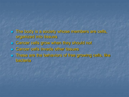
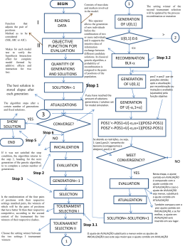
Cooperation and Conflict in the Evolution of Individuality. III.
Transitions in the Unit of Fitness
Richard E. Michod and Denis Roze
ABSTRACT. The evolution of multicellular organisms is the premier example of the
integration of lower levels into a single, higher-level individual or unit of fitness.
Explaining the transition from single cells to a multicellular organism is a major
challenge for evolutionary theory. We provide an explicit genetic framework for
understanding this transition in terms of the increase of cooperation among cells withingroups and the regulation of conflict within the cell group—the emerging organism.
Cooperation is the fundamental force leading to new levels of organization and selection.
While taking fitness away from lower level units (its costs), cooperation increases the
fitness of the new higher level unit (its benefits). In this way, cooperation may create new
levels of selection and higher levels of fitness. However, the evolution of cooperation sets
the stage for conflict, represented here by the increase of deleterious mutants during
development. The evolution of a means to regulate this conflict is the first new function
at the organism level. The developmental program evolves so as to reduce the
opportunity for conflict among cells. An organism is more than a group of cells related by
common descent; to exist organisms require adaptations that regulate conflict within.
Otherwise, continued improvement of the organism is frustrated by within-organism
variation and change during development. The evolution of modifiers of within-organism
change are a necessary prerequisite to the emergence of individuality and the continued
well being of the organism. Heritability of fitness and individuality at the new level
emerge as a result of the evolution of organismal functions that restrict the opportunity
for conflict within and ensure cooperation among cells. Conflict leads—through the
evolution of developmental adaptations that reduce it—to greater individuality and
harmony for the organism.
1. Introduction
1.1. Fitness. Lewontin once remarked that evolution by natural selection should
explain “fitness” [29]. In a recent book [39], one of us has taken the approach that to
explain fitness we need to understand three things: (i) how fitness originated in the
transition from the non-living to the living, (ii) the role of fitness in the mathematical
theory of natural selection, and (iii) how new levels of fitness are created during
evolutionary transitions to greater levels of complexity. The present paper is concerned
with the last question, and in particular how fitness emerges at the level of the
Mathematics Subject Classification. 92D15, 92C15. The authors appreciate the
comments of C. Lavigne and C. Nehaniv and the support provided by grants from
the NSF (DEB-95277716) and the NIH (GM-55505).
2
RICHARD E. MICHOD AND DENIS ROZE
organism out of a group of independently replicating cells. More generally, we are
interested in understanding evolutionary transitions to higher levels of organization
and complexity. Although, we primarily address the transition from single cells to
multicellular organisms, we believe our results are applicable to other evolutionary
transitions, such as the transition from replicating genes to cooperating gene networks,
from gene networks to the origin of the first cell, from bacteria cells to eukaryotic cells,
and the transition from multicellular organisms to societies.
1.2. A scenario for the origin of multicellular life. To help fix ideas, let us
consider a scenario for the initial stages of the transition from unicellular to
multicellular life (Figure 1).
Figure 1. Scenario for the first organisms (groups of cells). Shown in the figure are motile cells
with a flagella, non-motile mitotically dividing cells and cells which have yet to differentiate
into either motile or mitotic states. Because of the constraint of a single microtubule organizing
center per cell, cells cannot be motile and divide at the same time. As explained in the
accompanying text, motile cells are an example of cooperating cells and mitotically reproducing
cells are an example of defecting, or selfish, cells.
In simple multicellular organisms like Pleodorina in the Volvocales [5] or the
sponge Leucosolenia [9], the organism is a hollow sphere with at the top a fixed
proportion of cells remaining ciliated and dying at the end of the life cycle; the other
cells keeping the capacity to divide. We assume that reproduction and motility are two
basic characteristics of the early single celled ancestors to multicellular life, and these
single cells were able to differentiate into reproductive and motile states [9,30-32]. Cell
3
EVOLUTIONARY TRANSITIONS IN FITNESS
development was likely constrained by a single microtubule organizing center per cell,
and, consequently, there would have been a trade off between reproduction and
motility, with reproductive cells being unable to develop flagella for motility and
motile cells being unable to develop mitotic spindles for cell division [9,30,31]. Single
cells would switch between these two states according to environmental conditions.
Finally, the many advantages of large size (escape from predators being just one
possible advantage [6,19,46,47]) might favor single cells coming together to form cell
groups. We imagine the appearance of a new mutation perhaps coding for a cell
adhesion molecule or the collar structures that hold cells together in a Proterospongia
colony [27]. It is at this point that our investigations begin.
If and when single cells began forming groups, the capacity to respond to the
appropriate environmental inducer and differentiate into a motile state would be costly
to the cell, but beneficial for the group (assuming it was advantageous for groups to be
able to move). Because having motile cells is beneficial for the group, but motile cells
cannot themselves divide, or divide at a lower rate within the group, the capacity for a
cell to become motile is a costly form of cooperation, or altruism. Loss of this capacity
is then a form of defection, as staying reproductive all the time would be advantageous
at the cell level (favored by within-group selection), but disadvantageous at the group
level (disfavored by between cell-group selection). We are lead, according to this
scenario (and many others), to consider the fate of cooperation and defection in a
multi-level selection setting during the initial phases of the transition from unicellular
life to multicellular organisms.
1.3. Cooperation and conflict. New evolutionary units begin as cooperative
groups of existing units. Cooperation is the primary creative force in the emergence of
a new unit of selection, because it trades fitness at a lower level (its costs) for increased
fitness at the group level (its benefits). In this way, cooperation can create new levels of
fitness (Table 1). Two issues are central to the creation of a new unit of selection—
promoting cooperation among the lower level units in the functioning of the group,
while at the same time mitigating the inherent tendency of the lower level units to
compete with one another through frequency dependent fitness effects.
Cooperation
Cell
Level of Selection
represents the benefit of
Behavior
Cell
Group (organism)
group living; groups of
Defection (+) replicate faster
(-) less functional
existing
units
can
or survive better
behave in new and
Cooperation (-) replicate slowly
(+) more functional
useful ways. Frequency
or survive worse
dependent interactions Table 1. Effect of cooperation on fitness at cell and organism
among
evolutionary level. The notation +/− means positive or negative effects on
units are both a source fitness at the cell or organism level.
of novelty for the group
as well as a threat to its collective well-being. Cooperation is usually costly to the
fitness of the individuals involved. Defection (that is, non-cooperative behaviors) may
reap the benefits of the cooperative acts of others and spread in the population, thereby
destroying the very conditions upon which its spread depended in the first place. As a
result of the spread of defection, cooperation is lost and so is any hope for the creation
of a new higher level. Certain conditions are required to overcome the inherent limits
posed by frequency dependent selection to the emergence of new levels of selection:
4
RICHARD E. MICHOD AND DENIS ROZE
kinship, population structure, and conflict mediation. Conflict mediation is the process
by which lower level change is modulated in favor of the new emerging unit. The
definition or usage of certain fundamental terms and concepts used in this paper are
given in Table 2.
Term or Concept
Self-replication
Individual
Fisherian Fitness
Cooperation
Frequency
Dependent Selection
Conflict
Definition and Usage
The capacity to make copies, so that even mistakes can be copied
A unit of selection satisfying Darwin’s three conditions of variation,
heritability and self-replication with mechanisms to modulate lower
level change
Per capita rate of increase of a variant
An interaction that possibly decreases the fitness of the individual while
increasing the fitness of the group
When fitness depends upon interactions within a group or population
Competition among lower level units of selection leading to defection
and a disruption of the functioning of the group
Selfish Mutation
Mutations that are deleterious at the organism level and advantageous
at the cell level (as opposed to mutations that are deleterious at both
levels)
Conflict Mediation
The process by which the fitnesses of lower level units are aligned with
the fitness of the group
Fitness Covariance
The covariance between individual fitness and heritable genetic
properties (used to study the emergence of individuality)
Table 2. Definitions and usage of terms and concepts used in the paper.
1.4. Multi-level selection. A recent commentary on multi-level selection theory
observes whether there is anything in biology that can’t be explained by individual
selection acting on organisms, that requires selection acting on groups [41]. Although
rhetorical, this remark reflects a view often taken in biology that most interesting
questions can be addressed by viewing organisms as the sole unit of selection. But
where do organisms come from? From single cells, of course. And what are
multicellular organisms but cooperative groups of cells related by common descent. In
this paper, we extend a multi-level selection framework recently developed to study the
evolutionary transition from single cells to multicellular organisms [36]. We argue that
multi-level selection theory is needed to explain the origin of the organism—that very
creation which is supposed to deny the usefulness of multi-level selection in
evolutionary biology.
Organisms can be thought of as groups of cooperating cells. Selection among
cells could destroy this harmony and threaten the individual integrity of the organism.
For the organism to emerge as an individual, or unit of selection, ways must be found
of regulating the selfish tendencies of cells while at the same time promoting their
cooperative interactions.
During the proliferation of cells throughout the course of development,
deleterious mutation can lead to the loss of cooperative cell functions (such as the
ability to become motile in the scenario above). We represent cell function in terms of a
single cooperative strategy. Because deleterious mutation leads to the loss of cell
function, mutation may produce defecting cells from cooperative cells. Mutant cells no
longer take time and resources to cooperate with other cells and as a result may
5
EVOLUTIONARY TRANSITIONS IN FITNESS
replicate faster or survive better than cooperating cells. Such mutations are
disadvantageous at the organism level, but advantageous at the cell level. Deleterious
mutation can also produce completely defective cells with no capacity to replicate or
survive. Such mutations are disadvantageous at both the cell level and the level of the
group. In previous papers, we considered only defecting mutations, however, in the
present paper we consider both kinds of mutations. We also extend the multi-level
selection framework developed previously [36] by considering other forms of
reproduction involving fragmentation in addition to zygote based reproduction, because
we wish to understand the origin of the single cell stage which is almost universal in
the life cycles of complex organisms. In addition, we have discovered new equilibria
for the model at which linkage disequilibrium is positive and at which the population
is polymorphic for conflict mediation; for example, cell groups with and without a
germ line may coexist.
2. Multi-level Selection Model
2.1. Overview. The sequence of life cycle events involve the creation (through
gamete production or fragmentation or aggregation) of a founding propagule or
“offspring” group of cells of size N. These offspring grow and develop into an adult
and the adult then produces the offspring of the next generation. An overview of the
model life cycle is given in Figure 2. In the case of single cell reproduction considered
previously [36,37,39,40], N = 1, and sex (fusion and splitting with recombination) may
occur among offspring propagules.
Wj
'
q j , k ij
qj
qj
Figure 2. Model life cycle for the origin of organisms. The subscript j refers to the number of
cooperating cells in a propagule; j = 0, 1, 2, ...N, where N is the total number of cells in the
offspring propagule group, assumed constant for simplicity. The variable kij refers to the number
of cells of type i (either type C or D) in the adult cell group (that is after development) produced
by a propagule of type j. The variables qj (qj = j/N ) and q'j 4q'j = kCj k j 9 refer to the frequency
6
RICHARD E. MICHOD AND DENIS ROZE
of cooperation before and after development, respectively, while ∆qj is the change in gene
frequency at the C/D locus during development. Wj is the fitness of group j, defined as the
expected number of propagules produced by the group, assumed to depend both on size of the
adult group after development and its functionality (or level of cooperation among its component
cells) represented by parameter β in the models below.
After formation of the offspring, cells proliferate during development to produce
the adult form. This proliferation and development is indicated by the vertical arrows
in Figure 2. Because of mutation and different rates of replication of different cell
types, there will be a change in gene and genotype frequency of cells within-organisms
represented by ∆qj in Figure 2. There will also be a change in gene frequency in the
population due to differences in fitness between the adult forms. These two components
of frequency change, within-organisms and between-organisms give rise to the total
change in gene frequency ∆q. The number of cooperating and mutant cells of type i in
the adult stage of a j offspring is represented by the variables kij Figure 2. A model to
calculate these numbers is given below in Figure 3 and Table 3. The fitness of the adult
form, W j , is the absolute number of offspring produced and this is assumed to depend
both upon the number of cells in the adult and how the cells interact. Cooperation
among cells increases the fitness of the adult (parameter β in the models below) but
non-cooperating cells may replicate faster, survive better, and produce a larger but less
functional adult. Organism size is assumed to be indeterminate and to depend on the
time available for development as well as rate at which cells divide. Determinate size
can also be modeled. The evolution of conflict and cooperation in organisms with a
fixed size can be studied by standardizing the frequencies before offspring propagule
production much as is done in models of hard and soft selection [52].
2.2. Within-organism change. There are two components of gene frequency
change: (i) between-organisms within populations, and (ii) between-cells withinorganisms. In this subsection we
mutation rate from C to D per cell
µ
consider a model of within-organism
division
change stemming from mutation
t
generation time (for development)
during cell division and selection
c
rate of cell division for cooperating cells
among cells caused by differences in
b
effect of mutation on cell replication rate
cell replication or cell survival. The
cb
rate of cell division for mutant cells
basic variables are defined in Table 3
sC sD probability of cell survival for C and D
and explained in Figure 3.
cells, respectively
As cells proliferate within the
ct
k
= j 2sC 11 − µ 6
Cj
developing organism (development
time t) , mutations (rate µ ) occur
ct
x −1
b1 ct − x 6
=
j
µs D 2 s D
2 2sC 11 − µ 6
leading to loss of tissue function and
∑
k Dj
x =1
cooperativity among cells. We
bct
+1 N − j 6 2sC
consider only mutations that lead to a
loss of cooperation (C to D) not its
= k Cj + k Dj
kj
gain (no back mutation from D to C)
Table 3. Mutation and cellular selection model
as this represents a worse case for the
for haploidy. See also Figure 3 for an explanation
evolution of cooperation. This is
of how the numbers of different cell types in the
reasonable for biological reasons,
adult stage are calculated. Based on model of
because it is far easier to lose a
[42].
7
EVOLUTIONARY TRANSITIONS IN FITNESS
complex trait like cooperativity among cells than it is to gain it.
Within-organism variation after development is represented by the expected
number of cells of different types in the adult form—the kCj and kDj variables given in
Figure 2 and defined in Figure 3 and Table 3. Many aspects of the analysis, the various
equilibria and their stability for the different reproductive systems, can be obtained
analytically without explicitly specifying values for these variables. However, more
quantitative analyses require a specific within-organism mutation selection model. The
model of within-organism variation and selection presented in this section is a first
attempt at such a model. It has the virtue of being comparatively simple, at least in
principle, although it becomes complex computationally. There may be other more
realistic mutation selection models that could be used to obtain values for the kij
variables, and the model proposed in the last section was set up with this in mind.
0 5
ct
Figure 3. Calculation of the
Adult. The figure explains
the calculation of the
C
D
D
number of defecting cells
(D) in the adult stage
descended from a single
cooperate (C) cell in the
offspring propagule (formula
given in Table 3). For any
single cell generation we
assume replication, mutation
cell divisions
and then survival. A C cell
divides for x-1 divisions and
then mutates to D during cell
division x. Assume there are
Nx cells in generation x.
After cell division there are
2Nx cells and these survive
x 1 with probability sC or sD , for
C and D cells, respectively.
C
The total number of D cells
in the adult organism is
represented by the color
black in the adult form.
- 1 d ivisions
Consider C cells that have
divided, survived and not yet
mutated for x-1 divisions
and are now in the process
0
x-1
of cell division x. The total number of these cells is 2[2sC (1-µ)] . Some of these cells (µ) will
mutate for the first time and the resulting mutants will survive to the next cell division with
probability sD and then undergo b(ct-x) more cell divisions. We would like to choose the fitness
effect of the mutation at the cell level (b and sD) from a probability distribution of mutational
effects, but for the deterministic treatment given here these mutational effects are fixed
parameters of the model and the same for all mutations. The time taken to get x cell divisions is
x/c. The time left is t-x/c . The number of cell divisions the mutant will undergo is then cb(t-x/c)
= b(ct-x). The sum is over all possible cell divisions x. The formulae in the figure simplify to
∑2 2 s 1 − µ
x −1
µs
b c t −x
2s
t
b ct
t−
x
x
x
s
D
µ
C
2 2s 1 −µ
x
C
8
RICHARD E. MICHOD AND DENIS ROZE
those published previously, if there is no selection on cell survival, sC = sD = 1 [38]. This
approach gives k Cj , k Dj in Table 3 and Table 4 below.
The mutation model given in Table 3 and Figure 3 generalizes to the diploid case
following the arguments given elsewhere for a similar model but one without
differences in cell survival [37]; however the details are more complex and the steps
involved are not presented here for reasons of space. For example, to study the
branching process of mutations within cell lineages which start out as a CC cell
requires considering four classes of events: (i) CC cells that mutate to CD during cell
division x and then mutate to DD during cell division y, (ii) CC cells that mutate to CD
during cell division x and remain CD for the rest of development, (iii) CC cells that
mutate directly to DD during cell division x and, of course, (iv) CC cells that remain
CC for all of development.
The number of cells in an adult depends on the time available for development,
the rate of cell division and cell death. Rates of cell division vary widely among tissue
types. In some tissues cells stop dividing (brain, muscle, liver) while in other tissues
cells continue to divide throughout life (blood, intestine lining). To help fix ideas we
can estimate the number of cells that exist after a given development time, t, for
cooperating cells as follows. Ignoring mutation, cell death, and the different rates of
replication of the different cell types, t = 40 would allow 40 cell divisions (assuming c
= 1) implying around 1012 cells in the adult—a number similar in magnitude to the
number of cells in an adult human. Including cell death would require a greater
number of divisions to get the same number of cells in the adult. Cell death is likely
present in most cell lineages. For example, it has been estimated that the number of
cell divisions between the zygote and an average human male sperm is around 400 cell
divisions [51]. Such a large number of cell divisions is needed to account for cell death.
A typical human female egg is separated from the zygote by about 20 cell divisions
[51].
2.3. Mutation. Because there are two levels of selection, there are two levels at
which to consider the effects of mutation—the cell and the cell-group, or organism.
The mutations we consider always lead to the loss of the cooperative function, that is
the loss of the benefit β at the group level. This loss may be a pleiotropic consequence
of the disruption of other cell functions not directly related to cooperation. In this case,
the loss of cooperation may also be deleterious at the cell level, if these functions are
important for replication and survival of the cell. We refer to such mutations as
uniformly deleterious. According to the relative magnitude of the deleterious effects at
the two levels (β and b in the simplest model), uniformly deleterious mutations are best
eliminated by within-organism (between cell) or between-organism selection (see
Figure 5 below and accompanying discussion).
However, the loss of cooperation may not be a pleiotropic consequence of the loss
of cell functions related to cell fitness. Indeed, in Figure 1, mutant cells that are
defective in the capacity to differentiate into the motile state may replicate faster or
survive better than cooperating cells (because of the constraint of a single microtubule
organizing center per cell). By freeing energy or time spent on cooperation, the loss of
cooperation may lead to an increase of fitness at the cell level. Such selfish mutations
are deleterious at the organism level but advantageous at the cell level. Selfish
mutations are only eliminated by between-organism selection, because they are favored
by within-organism selection at the cell level.
9
EVOLUTIONARY TRANSITIONS IN FITNESS
The model is constructed to study both selfish and uniformly deleterious
mutations by considering the effects of mutation on the replication of cells withinorganisms in terms of the parameters c and b in Figure 3 and Table 3 (or sC and sD if
effects on cell survival are to be considered). For purposes of discussion, we consider
only effects of deleterious mutation on the replication rate of the cell (parameters c and
b), but effects of mutation on survival rates can also be studied (parameters sC and sD, in
Figure 3 and Table 3). The case of altruism given in Figure 1 is modeled by assuming
that mutation produces selfish cells that replicate faster than cooperating cells (c = 1, b
> 1). The case of complete altruism occurs when cooperating cells are not able to
survive or replicate at all, but here we focus on intermediate cases of altruism. In
addition to the case of selfish mutations, we study uniformly deleterious mutations by
considering ranges of the b parameter from zero (completely defective mutants) to
unity (mutant cells replicate at the same rate as cooperating cells) (c = 1, 0 ≤ b ≤ 1).
The deleterious mutation rate in the model pertains to the loss of cooperation and
perhaps other functions that affect cell replication and/or survival. Although the model
considers a single locus affecting cell behavior, there are likely to be many loci that
affect tissue function and cooperativity among cells. For this reason, we like to think of
this single locus as representing the cumulative effect of deleterious mutation at all loci
leading to loss of cooperation. This is not realistic modeling but provides a better
understanding of what we would like the model to represent. The mutation rate
parameter in the model does not pertain to cells in modern multicellular organisms but
rather to cells on the brink of coloniality during the period in which multicellular life
first arose. Indeed, an earlier version of the model predicts that one of the ways of
coping with within-organism change is to select for modifiers that lower the mutation
rate [36,40]. Modifiers are genes whose effect is to change the value of one of the
parameters in the model, such as the mutation rate, or in Section 3 the number of cells
in a propagule group, or in Section 4 the parameters of within-organism change.
Consequently, the mutation rate in modern organisms likely results from the very
processes being modeled here. For these reasons, we consider mutation rates that are
high when viewed as pertaining to a single locus in modern organisms.
Modern microbes as diverse as viruses, yeast, bacteria, and filamentous fungi,
have a genome-wide deleterious mutation rate of 0.003 per cell division even though
they have widely different genome sizes and mutation rates per base pair [13]. For
independently acting mutations, a mutation rate of 0.003 yields a low value for the
mutation load; the average fitness is approximately e-0.003 ≈ 0.997 [22,23]. The genome
wide mutation rate in modern multicellular organisms is much higher than in
microbes, for example; Drosophila has a genome wide rate (expressed on a haploid
basis) of approximately 0.5. Of course, the “organism” we have in mind here is
nowhere near as sophisticated as Drosophila, being on the threshold of the transition
from unicellular to multicellular life. The mutation rate in modern microbes of 0.003
has been attained through the evolution of modifiers over billions of years; these
modifiers presumably balanced the benefits of reducing the mutation rate with the
physiological costs of doing so. For this reason, we think a much higher overall
deleterious mutation rate likely held for the unicellular progenitors of multicellular life.
2.4. Fitness. There are interesting issues in how to model fitness in simple protoorganisms. As already mentioned the fitness of the organism, or cell-group, W j , is
simple enough to define; following standard models in population genetics, we take it
10
RICHARD E. MICHOD AND DENIS ROZE
to be the absolute number of offspring groups produced. Likewise, the fitness of the
cell is straight-forward to define in terms of its rate of replication and survival. The
interesting issues concern the relationship between fitness at the two levels and the
dependence of organism (cell-group) fitness on the fitness properties of component
cells. Cooperation is fundamental to the emergence of cell groups and, so, we take
organism fitness to depend upon the level of cooperation among its component cells—
using terms of the form 1+ βq'j in the models below, where β is the benefit of
cooperation and q'j is the frequency of cooperative cells in the adult stage.
Cooperation among cells increases the fitness of the adult (parameter β) but noncooperating cells may replicate faster, survive better, and as a consequence produce a
larger but less functional adult. The question then concerns whether and how to
include the effects of organism (cell group) size in organism fitness. If we ignore the
contribution of group size to fitness, we may take W j = 1 + βq'j . The effect of organism
size in a j-organism (organisms that start out as propogules with j cooperating cells)
may be represented by the term k j N , where the total number of cells after
development is kj and N is the number of cells in an offspring propagule (Table 3). If
we include the contribution of group size, fitness of the organism may then be taken to
be the product of organism size and the effects of cooperation or W j = 41 + βq'j 9k j N .
We note that if there were no mutation, including the term k j N in the
expression of fitness would not cause any variation of fitness with N. If there were no
mutation, there would be no within-group variation in replication or survival rates and
the adult group size, kj, would be a linear function of its starting size, N,
4 k0
= N 2bct and k N = N 2ct 9 and so N would cancel in the expression for W j . For
example, considering just the size component of fitness, k j N , for ct = 3, with N = 50
the adult size is 50 × 23 = 400 and the organism fitness is 400 / 50 = 8 , and with N = 1
the adult size is 8 and the fitness 8 / 1 = 8 . Consequently, it is not true that just because
organism fitness is divided by N, selection will always act to reduce N, so as to increase
Wj .
We think it most appropriate to include group size in organism fitness, for simple
organisms on the threshold of multicellular life. However, constructing fitness in this
way, W j = 41 + βq'j 9k j N , underscores the lack of true individuality in these early cell
groups, since there is a direct contribution of cell fitness to organism fitness. Even in
the case of no interactions between cells, that is no cooperation or defection, if C and D
cells had different intrinsic rates of replication or survival, there would be different
sizes among cell groups and different fitnesses of these groups according to k j N .
Yet, these differences in group fitness would have nothing to do with the interactions
among the component cells. For individuality to emerge at the cell-group level, fitness
at the new level must be decoupled from the fitness of the component cells.
As individuality at the cell group level becomes better defined, we expect
organism size to be regulated by factors other than intrinsic cell replication rates.
Modifiers affecting propagule size are studied in 3 and those affecting within-organism
11
EVOLUTIONARY TRANSITIONS IN FITNESS
change and conflict are studied in Section 4. Conflict modifiers regulating organism
size are expected to evolve so as to remove one of the advantages of cell defection, that
advantage being larger groups (J. Li and R. E. Michod, unpublished results). By
forcing all organisms, to attain a constant size, regardless of their proportion of
cooperating and defecting cells, determinant size can be seen as an adaptation to
regulate conflict. With determinate size, organism fitness would no longer depend on
the term k j N .
The simple models considered here (Table 3 above or Table 5 below) assume a
linear dependence of adult fitness on numbers of cooperating cells in the group,
although more complex models could be easily incorporated into the framework
considered there. At some point in the evolution of organisms, tissue function and
interaction became so integral that the organism could not survive without it.
Representing this (zero fitness below a threshold level of cooperation) requires
nonlinear fitness models. Multiplicative models and other nonlinear formulations can
also be considered in the same framework and can be expected to affect the outcome of
the model, much as is the case in the theory of kin selection studied during previous
project periods (see, for example, [33,34]).
3. Origin of the Single-Cell Stage of the Life Cycle
3.1. Overview. We wish to understand why the life cycle of most multicellular
organisms passes through a single cell stage. This single cell stage is present in a wide
variety of plants, animals, and fungi, from simple multicellular organisms in the
Volvocales to complex animals such as humans. We follow the terminology proposed
by others and use the word “zygote” to refer to the single cell produced during sexual
life cycles and the word “stem cell” to refer to the single cell produced during asexual
life cycles [15]. Our initial modeling framework involves asexual life cycles and the
origin of the stem cell. However, our longer term goal is to study sexual life cycles. To
understand why most life cycles involve a single cell stage we must consider alternative
forms of reproduction such as fragmentation (as occurs in Hydra [8], in colonial
choanoflagellates such as Proterospongia [27], or in colonial green algae [6]),
vegetative reproduction (as occurs in many plants) or aggregation (as occurs in the
social Myxobacteria and in the cellular slime molds). As already mentioned, we use the
word “propagule” to refer to the offspring of a reproductive process in which a sample
(assumed below to be of size N ) of cells is taken from the adult to produce the next
generation. The way in which the sample is taken affects the level of variation between
and within-groups (binomial sampling is assumed below for simplicity).
As discussed in the previous section, organisms are viewed as groups of
cooperating cells. As cells divide the group increases in size and propagule groups may
fragment off giving rise to the offspring of the next generation. Although, this may
happen continuously, for mathematical simplicity a discrete generation approach is
taken initially. Organisms (cell groups) are assumed to be composed of cooperating
cells (for example motile cells as in Figure 1) and mutant cells. Mutant cells may be
completely defective in all functions or defective in the capacity to differentiate into the
motile state, as considered in the motivating scenario given in Figure 1. Offspring
propagules are denoted by the number of cooperating cells in the propagule group, j =
0, 1, 2, ...N, where N is the number of cells in the offspring propagule group, assumed
12
RICHARD E. MICHOD AND DENIS ROZE
constant for simplicity. The problem of the evolution of single-cell reproduction is
basically the problem of the reduction of N to N = 1.
During development deleterious mutations (C to D) occur at rate µ. These
mutations may be caused by errors in DNA replication (genetic mutations) or errors in
the chromosome marking systems. Because the framework for individuality considered
here involves two levels of selection, the cell and the group or whole organism (see
Figure 1 and Figure 2), mutation may have deleterious effects at either level (or both).
Deleterious mutation may lead to the loss of the benefits of cooperation at the cell
group or organism level (for example, loss of motility or the capacity to respond to the
motility inducer as in Figure 1), or to the loss of other cell functions related to cell
replication and survival (as modeled by effects on the cell replication and survival
parameters in Figure 3 and Table 3. The number of cooperating and mutant cells in the
adult stage of a j propagule is k Cj and k Dj . A model to calculate these numbers is
given in Figure 3 and Table 3 above.
3.2. Propagule model There are assumed to be two alleles, cooperate C and mutant
D. The notation D is for Defect to describe the interesting case of selfish mutations that
lead to the loss of cooperation with enhanced rates of cell replication or survival.
However, deleterious mutations that disrupt cell function at both the level of the group
and the cell are also studied as described in the last section.
We refer to “organisms” in terms of the composition of the offspring with regard
to the number of cells that are cooperative at the cooperation locus. Because of withinorganism mutation and selection during development, the adult stage may have cells
that differ genetically from those in the offspring. The k-variables in Table 4 refer to
numbers of cells of
i,j
number of cooperating cells in offspring propagule
different genotypes in
group i, j = 0, 1, 2, ...N
the adult stage. There
N
number of cells in the offspring propagule group,
are two forces that may
assumed constant for simplicity
change gene frequency
xi
frequency of propagules with i C cells at time t
between the zygote and
frequency of propagule i produced from the adult
f ij
adult
stages
and
form of propagule j
determine the values of
kCj
number of C cells in the adult stage of a j-propagule
the
k-variables:
kDj
number of mutant cells in the adult stage of a jmutation and cellular
propagule
selection.
Mutation
kj
total number of cells in adult stage of j-propagule
after development, k j = kCj + k Dj
leads to the loss of
cooperation, and other
Wj
adult fitness (expected number propagules) of a jaspects
of
cell
propagule taken in Section 3 to be either
function.
Mutation
kj
W j = 1 + βq'j or W j = 41 + βq'j 9
, depending on
increases the variance
N
among cells withinwhether we assume that adult fitness depends on
organisms
and
adult size (see subsection 2.4 for discussion)
benefit to adult organism of cooperation among cells
enhances the scope for
β
freq. in adult and offspring for C gene for propagules
selection and conflict
q'j , q j
of type j
among cells. Cellular
'
q , ∆q freq. and change in freq. of C gene in total
selection is assumed to
population
depend on differences
Table 4. Haploid Propagule Model.
in cell survival or the
13
EVOLUTIONARY TRANSITIONS IN FITNESS
rate of cell replication (Table 3, Figure 3). The definition of terms and variables in the
haploid model is given in Table 4. Diploidy has also been considered previously in a
simpler model [37], but here we focus on the haploid case. With these definitions it is
straight forward to write down the new frequency in the next generation of propagules
of type i (given in Equation 1),
x i' =
N
Wj
∑ f ij W
j =0
xj ,
Equation 1
N
with W = ∑ Wi x i .
i =0
3.3. Modes of fragmentation. The parameter f ij is the frequency of type i
propagules among the offspring of a type j organism. This frequency depends on the
fragmentation mode considered. Kondrashov has studied the mutation load (defined as
the difference in average fitness with and without mutation) in a population where the
individuals produce offspring composed of N cells (as in our model) [26]. The model
that he used is similar to ours, but he doesn’t include within-organism selection. He
considers four possible modes of fragmentation (see his figure 1 [26]).
False mode: the N cells of each offspring are as genetically closed as possible. In
fact this case is equivalent to a single-cell-stage, and N has no influence on the
mutation load.
Sectorial mode: the N cells come from the same sector; this means that they all
come from the same initial cell. One can calculate fij in the following way. The
number of cells in the adult that arise from each of the j initial C cells is
µ 2bct − 2ct (1 − µ )ct µ
kC = 2ct (1 − µ )ct +
, so the probability of choosing a sector that
−1 + 2b −1 + µ
jkC
. The probability of having an offspring with i
arise from a C cell is
jkC + ( N − j )2bct
C cells and N-i D cells is for i > 0: f ij =
jkC
jkC + ( N −
N
( q )i (1 − qC ) N − i ,
bct i C
j )2
with
2ct (1 − µ )ct
being the frequency of C cells among the cells arising from a C
kC
initial.
Random mode: the N cells are taken randomly from the adult. In this case we
have Equation 2.
qC =
−
N ' i
' N i.
3 q j 8 31 − q j 8
i
fij = Equation 2
Recall, q'j is the frequency of cooperating cells in the adult form. The frequency
of C cells in the offspring and adult stage of a j offspring is q j = j N and
q'j = kCj
3 k Cj
+ k Dj 8 , respectively. The kCj and kDj variables are calculated Table 3 and
14
RICHARD E. MICHOD AND DENIS ROZE
Figure 3. To illustrate the model framework, we assume for simplicity Equation 2 that
involves random sampling across all cells in the adult form (with replacement). The
hypergeometric distribution would be more appropriate if the number of cells in the
offspring is big, but it can be approximated by a binomial distribution if the number of
cells in the offspring is small compared with the number of cells in the adult kj
(approximately N < kj/10).
Structured mode: each of the N cells come from a different initial cell (case 4).
Kondrashov shows that in this case the genetic load is maximal. We will consider the
sectorial and random cases in the analysis of the model.
To sum up, the different parameters of the model are represented in Table 3 and
Table 4. We note that this model could easily be modified to study the case of groups
formed by aggregation of cells (like slime molds). The model is deterministic and it
assumes an infinite population with discrete generations. Organisms are haploid and
asexual. Each organism begins its development with N cells. Cells can be of two types:
C (cooperative) or D (selfish with b > 1, or uniformly deleterious with b < 1). During
development, mutations C ‘ D occur at a rate µ per cell division. The parameters
representing the relative importance of intra- and inter-group selection are b and β.
Two modes of fragmentation are considered next (sectorial and random) in addition to
spore reproduction, and fitness may depend upon the size of the organism as well as on
the frequency of mutants in the organism.
3.4. Mutation load. Kondrashov calculates the mutation load (difference in
average fitness of populations with and without mutation) under vegetative
reproduction, using a similar model to ours but without including intraorganismal
selection [26]. Otto and Orive extended Kondrashov’s model to include
intraorganismal selection for uniformly deleterious mutations (they did not study
selfish mutations), and show that with moderate intraorganismal selection, the opposite
result obtains, that is mutation load decreases when N increases [42]. This indicates
that it can be advantageous to produce multicellular propagules if intraorganismal
selection can act upon the initial cell variants to eliminate mutations which are
deleterious at both levels. In Otto and Orive as in Kondrashov’s model, the fitness of
the organism doesn’t depend on its size (whereas it can in our model as discussed in
subsection 2.4). As we will see including organism size in organism fitness modifies
the results.
The model with N+1 recurrence equations 1 x 0 , x1 , ... x N 6 is too complex to be
treated analytically. Nevertheless Kondrashov shows that the mutation load at
equilibrium 3 L = 1 − W Wmax 8 can be calculated and is equal to 1 - O, O being the first
eigenvalue of the matrix f ijW j . The equilibrium distribution of the different types of
organisms is given by the first eigenvector of the matrix. He shows that the load
increases with N, and is more important with mode 2 of fragmentation than with mode
1, with the mode 3 than with mode 2 and with mode 4 than with mode 3 (1: false
mode, 2: sectorial mode, 3: random mode, 4: structured mode, see figure 1 of
Kondroshov [26]). This seems logical, indeed the variance between-organisms
decreases as N increases, and also from the mode 1 to the mode 4 of fragmentation,
and so selection is less effective at eliminating mutants.
15
EVOLUTIONARY TRANSITIONS IN FITNESS
There is no density-dependence in Kondrashov’s model: his recurrence equations
N
N
Wj
x j as in our
are written x i' = ∑ f ijW j x j (with constant W j ), and not x i' = ∑ f ij
W
j =0
j=0
model. So the matrix
f ijW j is the transition matrix of his system, whereas in our
model the transition matrix can be written
f ijW j W , W
changing at each
generation. Kondrashov’s model is linear, but not ours, and a priori we cannot use his
technique to calculate the mutation load and the distribution at the equilibrium.
Nevertheless, Cushing showed that in this particular case of non-linearity (when the
system can be written as the product of a scalar depending on the variables and of a
matrix independent of the variables), the equilibrium distribution is still given by the
first eigenvector of the matrix [11]. So we obtain the same frequencies at the
equilibrium with both models, and thus the same mutation load (this has been checked
by simulation).
Otto and Orive add to this model a kind of intraorganismal selection, with 0 < b <
1 (they don’t study the case of selfish mutants with b > 1). They show that the mutation
load increases with N only if the intraorganismal selection is weak (b close to 1). When
the within-organism selection is more important the results are opposite and the load
decreases when N increases. One can interpret this by saying that when the interorganism selection is important compared to the intra-organism selection, the mutants
are better eliminated when the variance between-organisms increases, whereas if the
intra-organism selection is more important the mutants are better eliminated when the
variance decreases (with more mixed groups).
Our preliminary results presented in subsection 3.5 confirm Otto and Orive’s
results, so long as there is no effect of organism size on fitness. However, when
organism size is included in organism fitness mutation load always decreases with
decreasing N. It is not clear in the work of Kondrashov [26] and Otto and Orive [42]
if the effects on mutation load are indicative of the direction of selection on genes
modifying the reproductive system by changing N. However, our results indicate that
modifiers for a single-cell stage of the reproductive cycle do the honorable thing and
increase when mutation load is decreased.
3.5. Preliminary results. We are currently investigating the equilibrium
distribution of propagule states. In Figure 4, the results of simulations of Equation 1
are given assuming binomial sampling as specified in Equation 2 and the mutation
selection model specified in Figure 3 and Table 3. The equilibrium frequency
distribution appears to qualitatively shift to a U-shaped distribution for small N from a
bell-shaped distribution for larger N. The U-shaped distribution is characteristic of loss
of intermediate states in which there are mixed groups of the two types of cells, while
the bell-shaped distribution is characteristic of maintaining intermediate mixed groups.
16
RICHARD E. MICHOD AND DENIS ROZE
This result anticipates a fundamental advantage (at least for selfish mutations) of
passing the life cycle through a bottleneck in cell number−increasing the variance at
the cell-group level and reducing the within-group variation and conflict. This favors
cooperation and helps to restrict the opportunity for defecting mutants to spread.
Notice that in Figure 4, the frequency of cooperation is much higher in panel A (N = 5)
than in panel B (N = 15). The limiting case of N = 1 corresponds to the transition from
fragmentation to spore production. A simple regulatory model has been proposed in
which the transition from fragmentation to spore production is caused only by a few
changes [48]. The origin of the single cell spore stage is a matter of great importance
for individuality and development.
As a first approach to the problem of selection on a modifier reducing propagule
size, we consider a population composed of two distinct reproductive types, a
“propagule reproducer” and “spore reproducer.” Propagule reproducers reproduce
according to the model given above (Equation 1 and Equation 2). There are N+1
recurrence equations for the propagule reproducer. The spore reproducer reproduces
according to the model studied in our previous work and requires just two equations,
since there are just two spore types for the haploid case, either C or D. The full vector
of state variables is then x ( 0),... , x ( N ), x ( C), x ( D) , with x(i) = frequency of
HT IUHT
HT IUHT
individuals without modifier with i non-mutant initial cells, x(C) = frequency of Cindividuals (with the modifier,
$ N = 5
starting their development with a
q
non-mutant cell), x(D) =
frequency of D-individuals (with
the modifier, starting their
development with a mutant cell).
An individual reproducing via
spores starts its development
SURSDJXOH FODVV
JHQHUDWLRQ
with only one cell and so the
number of cells in the adult stage
% N = 1 5
is lower than the number of cells
q
in the adult stage of an
individual without the modifier
(because t is the same for both
kinds of organisms). This can
have an effect on fitness,
nevertheless we don’t include
SURSDJXOH FODVV
JHQHUDWLRQ
this effect here. We have shown Figure 4. Simulation of propagule model for selfish
that the frequencies go to an mutations assuming W = 1 + βq ' k N . Using
j 4
j9 j
equilibrium given by the first
right eigenvector of the W j f ij
matrix (constructed in a similar
manner to Kondrashov [26] but
including the equations for the
spore reproducers).
Equation 1 and Equation 2. Parameter values in panel
(A): c = 1, t = 10, β = 3, µ = 0.003, b = 1.1; and in panel
(B): c = 1, t = 10, β = 10, µ = 0.01, b = 1.05. As
explained elsewhere [40] these parameter values are
appropriate for the transition involving cell groups
similar in size to some species of Volvocales. The
ordinate is either the equilibrium frequency of a
propagule class (“eq. freq.”) or the frequency of
cooperation, q.
17
EVOLUTIONARY TRANSITIONS IN FITNESS
U
1 O
DQG
RP
When mutations are selfish the spore reproducer always wins, because it is always
advantageous to increase the variance between-organisms (and there is no cost of doing
so because we have assumed no effect of N on adult size). This is always the case, for
both fitness functions in Table 4.
Results for uniformly deleterious mutations are given in Figure 5 for the two
fitness
functions:
when
$ ILWQHVV LQGHSHQGHQW RI JURXS VL]H
organism fitness is independent
of group size (panel (A)) and
when organism fitness depends
upon group size (panel (B)).
When fitness depends only on
the frequency of cells (Figure 5
panel (A)), we have found that,
when
the intraorganismal
1 selection is weak (b close to 1),
WRU DO
VH F
the spore reproducer
is
selected, because betweenb
organism selection is more
effective at eliminating the % ILWQHVV GHSHQGV RQ JURXS VL]H
deleterious mutations. When
intraorganismal
selection
FW
becomes stronger, the spore
VH
reproducer is no longer
selected. We have studied the
1
critical value of b for single
cell (spore) reproduction to be
selected, for several values of
the other parameters. In Figure
5, this critical value of b occurs
when the N = 5 curve intersects
b
the N = 1 curve (at a value of b Figure 5. Mutation load (1- λ) and selection on spore
slightly greater than b = 0.95 (stem cell) reproduction for mutations deleterious at both
in the figure). The critical levels of selection. Parameter values are µ = 0.003, t = 20,
value of b doesn’t change much β = 3. The parameter b on the abscissa is the replication
when the value of N for the rate of mutant cells. Non-mutant cells replicate at rate 1.
propagule reproducer changes. Spore production is always selected for selfish mutations
In other words, the condition (b > 1). In panel (A), spore reproduction (N = 1) wins
for
selection
of
spore when the mutation load decreases with N (to the left of the
reproduction is about the same point where the solid line crosses the others). Key in both
regardless of the size of the panels: dashed lines for N = 5 and random mode of
propagules of its competitor. In fragmentation (Equation 2); dotted lines for N = 5, and
addition,
the
mode
of sectorial mode of fragmentation; solid lines for N = 1. The
fragmentation has a small, but differences between the panels involve the way in which
barely noticeable effect, on this fitness is modeled at the organism (cell-group) level. In
critical
value.
As
just panel (A) fitness is independent of group size
mentioned, the curves for other W = 1 + βq' , while in panel (B) fitness depends on group
j
j
values of N > 1 intersect
approximately at the same size Wj = 41 + βq 'j 9 k j N . See text for explanation.
DO
L
RU
DQ
U
1 O
GR
P
L
18
RICHARD E. MICHOD AND DENIS ROZE
point and behave qualitatively as does the N = 5 curve in that mutation load is greater
(or smaller) than the N = 1 curve when b is to the right (left) of the intersection.
Consequently, the main result concerning the evolution of spore reproduction when
fitness is independent of group size is that, when the mutation load increases with N
(to the right of the point at which the curves intersect in panel (A) of Figure 5), the
modifier is selected (the spore reproducer wins); and when the mutation load decreases
with N (to the left of the point of intersection), the modifier is not selected (the
propagule reproducer wins).
However, when organism fitness depends upon group size, as it should for simple
groups on the threshold of multicellularity, mutation load always decreases with N, and
the spore reproducer is always selected (Figure 5 panel (B)). For the values of b lower
than 0.8 the value of the load almost doesn’t depend on N. Indeed the betweenorganism selection is reinforced by the effect of size (the more the proportion of
deleterious mutants is important, the smaller is the organism). For the values of b
lower than 0.8 the proportion of mutants in the population is low, whatever the value
of N.
Under the sectorial mode of fragmentation, all cells of a propagule come from the
same initial cell in the parent. The kinship among cells in the propagule is higher, and
the variance between-organisms is higher, under sectorial sampling than under random
sampling. As we see in Figure 5 (panel (A)), when the between-organism selection is
more effective at eliminating deleterious mutations (b less than but close to unity), the
mutation load is greater with random sampling than with sectorial sampling. The
opposite result obtains when within-organism selection is more effective (b
significantly less than unity) and the mutation load is lower under random than under
sectorial sampling. When fitness depends upon group size (Figure 5 panel (B)), the
load is always greater under random sampling than under sectorial sampling.
There are other aspects of the single cell state that require serious consideration,
but these have been ignored here. First, there is the opportunity it provides to reset
development. The second aspect of the single cell state is its role in the sexual life
cycle. It is difficult to imagine sex between-organisms that does not involve a single
cell state.1 We intend to address these viewpoints in due time.
4. Evolution of Conflict Mediation
4.1. Overview. The preliminary results reported in the last section lend credence
to the view that, by passing the life cycle through a single cell stage (the stem cell,
spore or zygote), the opportunity for between-group selection is enhanced while the
opportunity for within-group conflict is reduced. This can favor the transition between
single cells and cell groups. We now (and in the next section) consider further aspects
of the transition from single cells to organisms by assuming throughout section 4 that
1
Perhaps, bacterial transformation or recombination in viruses (such as occurs during multiplicity reactivation)
comes closest to the case in which recombination may occur among DNA molecules from multiple partners. In the
slime mold, spores from a single individual may involve mating and recombination of cells from different parents.
In the life cycle of the slime mold Dictyostelium discoideum, the single cell products of the organism, the spores,
form amoebae that ultimately aggregate in groups to form a new multicellular individual, first the migrating slug
and then the fruiting body. During the single cell amoebae stage before aggregation, sex (fusion and meiosis) may
occur (for review see [50]). As a consequence, a single individual (fruiting body) may involve cells that are
recombinations among different parent cells (the degree to which this occurs depends upon the relatedness of the
aggregating cells).
19
EVOLUTIONARY TRANSITIONS IN FITNESS
cell groups originate from single cells. In our view an organism is more than a group
of cooperating cells, more even then a group of cooperating cells related through
common descent from a single cell. An organism must have functions that maintain its
integrity and individuality. We are interested in understanding the first true emergent
level functions during the emergence of the first true individual, the multicellular
organism.
All models make assumptions about the processes they study, in the present case,
these assumptions involve parameters representing within-organism mutation and cellcell interaction during development. The purpose of the modifier model introduced
here is to study how evolution may modify these assumptions and parameter values,
and further how these modifications affect the transition to a higher level of selection.
Unlike the classical use of modifier models, say in the evolution of dominance and
recombination, the modifiers studied in the present paper are not neutral. Instead, they
have direct effects on fitness at the cell and organism level by changing the parameters
of within-organism change. By molding the ways in which the levels interact so as to
reduce conflict among cells, for example by segregating a germ line early or by
policing the selfish tendencies of cells, the modifiers construct the first true emergent
organism level functions.
4.2. Model parameters. Recall the parameters of the model studied above. These
parameters describe fitness effects at the organism (β) and cell level (b, sC, sD), the
mutation rate per cell division (µ) and the development time (t). The parameter β is the
benefit to organism fitness of cooperation among its component cells. Fitness is
assumed to depend linearly (through β) on the number of cooperating cells in the
organism’s adult stage (see Table 5). The parameter bc is the replication rate of
defecting cells (c is the replication rate of cooperating cells, assumed equal to unity).
The parameters sC, sD are the survivals of C and D cells per cell generation (assumed
equal here for simplicity). The parameter µ is the rate of mutation per cell division
during development (interpreted here as the genome wide deleterious mutation rate at
all loci leading to a loss of cell function). The parameter t is the time available for
development (development allows for within-organism change resulting from
mutation, µ, and selection, b, sC, sD , at the cell level). A new parameter is needed in the
case of sexual reproduction with the possibility of recombination between two loci; r is
the rate of recombination between the cooperate/defect locus and the modifier locus.
Again, the complexity of interaction among different cell types and tissue functions is
assumed to be represented by two kinds of interactions—cooperate and not cooperate
(or defect). Heritability of fitness at the organism level is measured by the regression of
offspring fitness on adult fitness.
A per cell division mutation rate of µ = 0.003 is assumed in many of the studies
reported in this section. The reason for assuming this value has been discussed above,
in Section 2.3. Nevertheless, smaller mutation rates also result in the evolution of
modifiers of within-organism change (that is the transition from equilibrium 3 to 4
discussed below, see, for example, panels (D) and (E) of Figure 6). Higher mutation
rates mean more within-organism change and this facilitates evolution of the modifier.
4.3. Two-locus modifier model. We now consider a second locus which is
assumed to modify the parameters of within-organism change at the cooperate/defect
(C, D) locus (see Table 5 for the additional terms for the modifier model).
20
RICHARD E. MICHOD AND DENIS ROZE
The modifier locus is interpreted here as either as a germ line locus or a mutual
policing locus, according to whether the modifier allele M affects the way in which
cells are chosen for gametes (germ line modifier), or the parameters of selection, and
variation at the organism and cell level (policing modifier). A germ line modifier is
assumed to sequester a group of cells with shorter development time and possibly a
lower mutation rate than the soma and less selection at the cell level. A self-policing
modifier causes the organism to spend time and energy monitoring cell interactions
and reducing the advantages of defection at a cost to the organism. In either case, the
modifier locus is assumed to have two alleles M and m, with no mutation at the
modifier locus. Because there is no mutation at the modifier locus and groups start out
as single cells, there can
Variable Definition
be
no
within-group
i,j
indices for genotype 1, 2, 3, 4 = CM, Cm, DM,
change at the modifier
Dm
locus because there is no
kij
number of i cells in the adult stage (soma) of a jwithin-group variation at
zygote
the modifier locus. A
kj
total number of cells in adult stage (soma) of jgroup of cells expressing
zygote, k j = ∑ k ij
i
allele m is assumed to
K
i
number
of
cells
in the germ line of a j-zygote
ij
have the same properties
K
total
number
of
cells
in the germ line of j-zygote,
j
as the cell-groups studied
K
K
=
in the previous section
∑i ij
j
(assuming N = 1). A
Wj
individual fitness of j-zygote (assumed to depend
group of cells expressing
on group size): W j = k j + β 4 k1 j + k 2 j 8
allele M is assumed to
r
recombination rate between C/D and M/m loci
have different properties
x
frequency
of two locus j genotype in total
j
that represent the ideas of
population
a germ line or self
policing.
Table 5. Additional notation and terms for the two locus
The additional terms
modifier model. The genotype frequencies, xj, are measured at
and definitions for the
the gamete stage, before mating, meiosis, development and
two-locus modifier model
within and between-organism selection. The variables, xj, are
are given in Table 5.
now completely different than those defined in the propagule
Some explanation of the
model in Table 4. The table considers germ line modifiers that
haploid
life
cycle
create a separate germ and somatic line, each of which may
considered here may be
have different numbers of cell types (the Kij and kij variables).
helpful. In the diploid life
In the case of self-policing modifiers, there is no distinction
cycle,
a
generation
between the germ line and the soma (all cells are potential
typically begins with the
germ line cells).
diploid zygote, followed
by development, within and between-organism selection, the adult stage, meiosis and
the production of haploid gametes which fuse to produce the zygotes of the next
generation. In previous analyses of the two-locus haploid modifier model studied here,
it was also assumed that the generation began with the zygote stage (Michod 1996,
Michod and Roze 1997). In the haploid life cycle, the haploid zygote stage is followed
by development, within and between-organism selection, the adult stage (still haploid),
production of haploid gametes, fusion of gametes to produce a transient diploid stage
which undergoes meiosis to produce the haploid zygotes of the next generation.
Although it doesn’t affect the results, the two-locus recurrence equations are simpler
21
EVOLUTIONARY TRANSITIONS IN FITNESS
for the haploid life cycle, and easier to understand, if we begin a generation with the
gametes and let the xj variables be the frequencies of the different genotypes among
gametes (instead of among zygotes). Consequently, the following sequence of events in
each generation is assumed: gametes, fusion of gametes to make the transient diploid
stage, meiosis and recombination to form haploid zygotes, development, within and
between-organism selection to create the adult stage, and then formation of the
gametes to start the next generation.
The recurrence equations for the two-locus haploid life cycle may be constructed
as follows. Recombination may change the genotype frequencies according to the level
of linkage disequilibrium in the population. Linkage disequilibrium measures the
statistical association between the frequencies at the two loci. If G = 0, the joint
distribution of alleles in gametes is the product of the allele frequencies and
recombination has no effect on the genotype frequencies. In Equation 3, we define
linkage disequilibrium between the locus determining cell behavior and the modifier
locus (using the variable G for gametic phase imbalance).
G = x1x 4 − x2 x3
Equation 3
After meiosis, the frequencies of the four genotypes may change from what they were
before fusion, depending on the rate of recombination (r) and the level of linkage
disequilibrium, G. The new frequencies after recombination are x1 - rG, x2 + rG, x3 +
rG, and x4 - rG, for the CM, Cm, DM and Dm genotypes, respectively. It is upon these
new genotype frequencies that selection and mutation operate, as shown in Equation 4.
The full two-locus dynamical system is given in Equation 4,
K11
K1
K
x2' W = 1 x2 + rG 6W2 22
K2
x1' W = 1 x1 − rG 6W1
K31
K1
K
x 4' W = 1 x4 − rG 6W4 + 1 x2 + rG 6W2 42
K2
,
Equation 4
x3' W = 1 x3 + rG 6W3 + 1 x1 − rG 6W1
with
W = 1 x1 − rG 6W1 + 1 x 2 + rG 6W2 + 1 x3 + rG 6W3 + 1 x 4 − rG 6W4
and
linkage
disequilibrium given by Equation 3. Only three of the equations are independent, since
the frequencies must sum to one. Equation 4 gives the same results as the equations
studied previously (equations 1 and 2 of Michod 1996 and in Michod and Roze 1997).
The primary difference is that genotype frequencies are measured among gametes and
not zygotes, and this allows a simpler form of the recurrence equations.
4.4. Equilibria of the system. The transition to a new level of selection proceeds
in two general stages. First, cooperation must increase. Deleterious mutation leads to
the loss of cooperation. A mutation selection balance may be reached at which the
increase of cooperation (by group selection) is offset by its loss through mutation. As
discussed previously, the increase of cooperation within the group is accompanied by
an increase in the level of within-group change and conflict as mutation and selection
among cells leads towards defection and a loss of cooperation [37]. The second stage in
an evolutionary transition is the appearance of modifier genes that regulate this within-
22
RICHARD E. MICHOD AND DENIS ROZE
group conflict. Only after the evolution of modifiers of within-group conflict, do we
refer to the group of cooperating cells as an “individual,” because only then is the
group is truly indivisible in that it possesses higher level functions that protect its
integrity.
The main equilibria of the system of are given in Table 6. These equilibria are
obtained by setting linkage disequilibrium to zero (G=0, using Equation 3) and by
setting the change in genotype frequencies equal to zero (using Equation 4). The
equilibria given in Table 6 are the ones we expect based on the biological assumptions
of the model, however they assume that linkage disequilibrium (Equation 3) is zero. In
the case of germ line modifiers discussed in the next section, we have found examples
of other equilibria at which G ≠ 0 , but they are confined to narrow regions of the
parameter space. These equilibria with G ≠ 0 are, nevertheless, quite interesting as the
populations are polymorphic at the modifier locus and maintain both germ line and
non-germ line phenotypes in the same population.
Eq.
1
2
3
4
Description of Loci
no cooperation; no modifier
no cooperation; modifier fixed
polymorphic for cooperation and
defection; no modifier
polymorphic for cooperation and
defection; modifier fixed
Interpretation
Non-functional cell groups, single cells2
Not of biological interest, never stable
Groups of cooperating cells: no higher level
functions
Individual organism: integrated group of
cooperating cells with higher level function
mediating within-organism conflict
Table 6. Equilibria for modifier model without linkage disequilibrium. See especially Table A 1
and Table A 2, for a mathematical description of the equilibria and eigenvalues.
For the moment we focus on the equilibria given in Table 6. The eigenvalues of
the three independent genotypes 1 x 4 = 1 − x1 − x 2 − x3 6 are given in Table A 2 for the
different equilibria and for sexual and asexual reproduction. The evolution of
cooperation corresponds to equilibrium 3 and the evolution of the modifier corresponds
to equilibrium 4. Consequently, the question of the transition to individuality boils
down to the conditions for a transition from equilibrium 3 to equilibrium 4. The
condition for increase of the modifier is given as λ 31 in Table A 2. In the case of
asexual reproduction, λ 31 > 1 means that a CM organism must produce more C
gametes than a Cm organism.
The evolution of functions to protect the integrity of the organism are not
possible, if there is no conflict among the cells in the first place. It is conflict itself (at
equilibrium 3) which sets the stage for a transition between equilibrium 3 and 4 and
the evolution of individuality.
4.5. Evolution of the germ line. The essential feature of a germ line is that
gamete producing cells are sequestered from somatic cells early in development.
Consequently, gametes have a different developmental history from cells in the adult
form (the soma) in the sense that they are derived from a cell lineage that has divided
for a fewer number of cell divisions with, perhaps, a different mutation rate per cell
replication and a different selective context. The main parameters influencing the
2
The model assumes cell groups. Nevertheless, we think of Eq. 1 as representing single cells, because there is no
cooperation and no interaction between cells to maintain the group structure assumed in the model.
23
EVOLUTIONARY TRANSITIONS IN FITNESS
evolution of the germ line is the reduction in development time in the germ line
relative to the soma, δ (with the development time in the germ line being t M = t − δ ),
the deleterious mutation rate in the germ line, µM, and the nature of cell selection in the
germ line.
Adult
Stage
Genotype of Zygote
CM
Germ Cells, Kij
CM
2
ct M
bct M
−2
Somatic Cells, kij
ct M
11 −
b −1
−1 + 2
Dm
Cm
Dm
0
0
0
0
0
2bct
0
0
2bct
0
µM2
CM
DM
11 − µ M 6
Cm
DM
Cm
ct M
µM6
ct M
µM
+ µM
0
2
ct
ct
11 − µ 6
ct
2ct 11 − µ 6
0
ct
DM
µ 2bct − 2ct 11 − µ 6 µ
−1 + 2b−1 + µ
0
ct
µ 2bct − 2ct 11 − µ 6 µ
Dm
0
−1 + 2b−1 + µ
Table 7. Numbers of different cell types in the soma and gamete stages for germ line modifiers.
Zygote genotype is given across the top (column) and the genotype of the cells after development
is given down the rows. For genotypes containing the m allele, there is no germ line; so there is
no difference between the germ line stage and the somatic adult stage. The germ line is ignored
in D containing zygotes since by assumption there is no mutation from D to C and so no withinorganism variation in D containing zygotes. The steps involved in obtaining the formulae in the
table are described in Table 3 and Figure 3. We do not consider mutations at the germ line
locus, since we are interested in the loss of tissue function and cooperation among somatic cells.
A modification of the model given in the text relates the table to the study of a self-policing
allele. Selection is allowed in the germ line stemming from the different rates of replication of
cooperate and defecting cells. This makes matters more difficult for the origin of the germ line.
We also consider in Table 8 the case that, since germ line cells don’t cooperate and otherwise
function in somatic functions, the replication advantage of defecting cells no longer obtains in
the germ line.
We are interested in modeling the origin of germ cells in an ancestor that had
none. Furthermore, we wish to consider the hypothesis that the germ line serves to
increase the heritability of traits in the organism, as opposed to directly increasing
organism fitness. For this reason, we assume that the germ line is costly to fitness
(expected number of offspring) although it increases the heritability of fitness
(regression of fitness of offspring on fitness of parents). Where do the germ line cells
come from? We imagine that the total number of cells is conserved and allocated
between the germ line and the soma. Cells sequestered in the germ line are no longer
available for somatic function, and, for this reason, the germ line allele may detract
from adult organism function. One way of representing this cost is by subtracting the
24
RICHARD E. MICHOD AND DENIS ROZE
Germ Cells, Kij
germ line cells from the somatic cells in the adult form (kij - Kij in Table 7 and Table
8). The number of cells is directly related to the development time, t. So if δ is very
small, then the number of cells in the germ line is quite large leaving few cells for
somatic function. For this reason, we find that the transition from equilibrium 3 to 4
cannot occur by a continuous increase of δ from zero. There is a threshold value of δ
resulting from the cost of the germ line which must be overcome for the modifier to
increase. If there were no cost, the germ line allele always spreads in the population.
Adult
Genotype of Zygote
There is a limitation in our approach to
Stage
CM
modeling the origin of the germ line. Fitness is
ct
ct
assumed to depend on the number of cells in the
CM
2 M 11 − µ M 6 M
soma and not on the number of cells in the
Cm
0
germ line. Fitness is maximal when no cells are
ct
2ct M 1 − 11 − µ M 6 M allocated to the germ line, because there are
DM
more cells available for somatic function
Dm
0
(although the heritability of fitness is less, if
there is no germ line). Presumably, the number
Table 8. Numbers of different cell
of cells allocated to the germ line will have
types in the gamete stages for germ
some effect on the number of gametes produced,
line modifiers assuming no selection
but we have ignored the problem of modeling
in the germ line. See Table 7 for
this effect.
explanation of table. Only the CM
In Table 8 we give the numbers of zygote is shown here, the other zygotes
different cell types in the gamete stages for
have germ and soma properties as
germ line modifiers, assuming complete
specified in Table 7.
differentiation between germ and soma. In other
words, we assume that there is no expression of cooperate/defect phenotype in germ
line and so no selection in the germ line (b = 1 in the germ line). Deleterious mutation
may still occur in the germ line, however it is neutral at the level of the cell in the
germ line (mutation still disrupts cell function in the soma, however). We represent no
selection in the germ line by assuming b = 1 in the table cell corresponding to the DM
gametic output of a CM zygote. No selection in the germ line only makes sense for
selfish mutations (b > 1), since cells that are defective at both levels of selection (b < 1)
may be expected to replicate more slowly in both the germ and the soma because they
are generally defective (not just defective in the cooperative function).
We now return to considering the evolutionary equilibria of the system. The
equilibria of Equation 4 correspond to different evolutionary outcomes. Regions of
stability of the different equilibria for different parameter values are given in Figure 6
in terms of the reduction of development time caused by the germ line modifier, δ, and
the replication rate of mutant cells, b. The replication rate of cooperating cells is unity
(c = 1). Recall that mutations are beneficial (selfish mutants), neutral or deleterious at
the cell level when b > 1, b = 1, and b < 1, respectively.
The transition involving the increase of cooperation (Eq. 1 to Eq. 3 in Figure 6)
has been considered previously (Michod 1997a). This transition occurs for parameter
values in the regions marked Eq. 3 in the panels in Figure 6, while cooperation will not
increase for parameter values in the Eq. 1 region. The transition which interests us
here involves the increase of modifiers of within-group change and this transition
occurs after cooperation increases (Eq. 3 to Eq. 4 in Figure 6). The conditions under
which the population evolves from equilibrium 3 to 4 were studied previously [36].
This transition occurs for parameter values in the Eq. 4 regions in Figure 6. In a later
25
EVOLUTIONARY TRANSITIONS IN FITNESS
section (Transitions in Individuality), we study the components of this transition in
terms of the emergence of fitness and the heritability of fitness at the new organism
level.
β = 3 , t = 40, µ = 3 x10 -3
β = 3 0, t = 4 0 , µ = 3 x10 -3
$
%
δ
δ
20
20
Eq. 4
Eq. 4
15
15
10
Eq. 1
Eq. 3
5
10
Eq. 3
5
0.2
&
δ
0.4
0.6
0.8
1
1.2
b
0.2
β = 3 , t = 20, µ = 10 -3
20
17.5
15
12.5
10
7.5
5
δ
Eq. 1
Eq. 3
0.6
0.8
1
1.2
b
β = 3 , t = 20, µ = 10 -4
'
Eq. 4
0.4
Eq. 1
20
17.5
15
12.5
10
7.5
5
Eq. 4
Eq. 1
Eq. 3
2. 5
2. 5
0.2
(
δ
0.4
0.6
0.8
1
1.2
b
0.2
β = 3 , t = 20, µ = 10 -5
)
0.4
δ
Eq. 4
0.8
1
1.2
b
β = 3 , t = 10, µ = 3 x10 -3
10
20
17.5
15
12.5
10
7.5
5
0.6
Eq. 1
Eq. 4
8
Eq. 1
Eq. 3
6
Eq. 3
4
2
2. 5
0.2
0.4
0.6
0.8
1
b
1.2
0.2
0.4
0.6
0.8
1
1.2
b
Figure 6. Stability of evolutionary equilibria for germ line modifiers. Results here assume
selection in the germ line (Table 7). The modifier is assumed to decrease the development time
for the germ line (when compared to the soma) by amount δ. Selfish (b > 1) and uniformly
deleterious (b < 1) mutations are considered. Regions of stability for the different equilibria
described in Table 6 are given as a function of the replication rate of mutant cells (relative to
cooperating cells), b, and δ, for different values of the mutation rate, µ, development time, t, and
advantage of cooperation, β. Solid curves are for asexual reproduction and dashed curves for
sexual reproduction assuming a recombination rate of r = 0.25 between the modifier and
cooperate/defect locus. Cells sequestered in the germ line are not available for somatic function.
The mutation rate is assumed to be the same in the soma and the germ line. See also Figure 1 of
Michod [37] for more detailed treatment of the boundary between equilibrium 3 and 4 in three
dimensions (b, µ, δ).
26
RICHARD E. MICHOD AND DENIS ROZE
The general result apparent in Figure 6 is that the modifier increases for all kinds
of mutations at the cell level (beneficial, neutral or deleterious) so long as they are
deleterious at the organism level (as is assumed throughout) and the reduction in time
for replication, δ , is large enough. As the mutants change from being beneficial at the
cell level to deleterious, it becomes more difficult for the germ line modifier to
increase, in the sense of requiring a larger decrease in the time available for replication
in the germ line (all panels in Figure 6). Selfish mutants are most efficacious in
selecting for a germ line, nevertheless all mutations deleterious at the organism level
promote selection for the germ line modifier.
The parameters have understandable effects on the regions of stability of the
different equilibria described in Table 6. For example, as the benefit of cooperation to
the group increases from β = 3 to β = 30, larger replication benefits of defection at the
cell level are tolerated as shown in panels (A) and (B) of Figure 6. Likewise, as the size
of the organism decreases from t = 40 to t = 20 to t = 10 (shorter development times),
larger benefits of defection at the cell level are tolerated although the reduction in
development time for the germ line to evolve is about the same (see panels (A), (C) and
(F) of Figure 6). As the mutation rate decreases from 10-3 to 10-4 to 10-5, it becomes
more difficult for germ line modifiers to increase, in the sense that larger reductions in
development time are required for there to be a transition from equilibrium 3 to 4 (see
panels (C), (D) and (E) of Figure 6; see also Figure 1 of Michod [37]). Higher mutation
rates mean more within-organism change and this makes it easier for conflict
modifiers to increase.
Figure 6 shows the limits of these regions of stability of the four equilibria in
Table 6 in (b,δ ) space, for different values of the time for development, t , the benefit
of cooperation, β, and µ the mutation rate. Recall, the parameter δ is the difference
between the development time of the soma (t) and of the germ line. In the case of
asexual reproduction these different regions don’t overlap. With sexual reproduction,
there are regions in which more than one equilibrium can be stable at the same time
(bi-stability) and regions in
which none of the four
r = 0 .5 , β = 3 0, t = 4 0, µ = 3 x10
equilibria given in Table 6 are
stable. Such a situation is
ELVWDEOH
shown in Figure 7, for selfish
E q. 4
mutations (b > 1).
In Figure 7, there is
assumed to be no selection in
the germ line (Table 8),
E q . w ith G > 0
although
the
conclusions
E q. 1
discussed now also apply when
E q. 3
there is selection in the germ
line (Table 7). There are three
curves given in Figure 7 which Figure 7. Equilibria and regions of stability for germ line
overlap in different regions. modifier and selfish mutations. No selection in germ line
First there is a nearly vertical (Table 8), although the qualitative relationships of the
dotted line at about b = 1.1. To three curves (bi-stable and Eq. with G > 0 regions) are
the right of this line, similar if there is selection in the germ line (Table 7), or
equilibrium 1 is stable and if the recombination rate is smaller so long as r > 0. See
there is no cooperation among text for explanation.
-3
27
EVOLUTIONARY TRANSITIONS IN FITNESS
cells. Second there is a solid curve which defines the region of stability for equilibrium
3. Below this curve equilibrium 3 is stable and there is cooperation but the germ line
modifier won’t increase. Third, there is a dashed-dotted curve which defines the region
of stability for equilibrium 4. Above this curve equilibrium 4 is stable; both cooperation
and the germ line modifier are present.
The region in which both equilibrium 1 and 4 are stable is labeled bi-stable in
Figure 7. Depending on initial conditions the population can switch between no
cooperation to a fully functional organism. This requires the introduction of the two
alleles C and M at the same time and on the same chromosome. We consider this to be
a rare and unlikely event. Nevertheless this suggests that with sex, mixed populations
of individual cells (no organisms, Eq. 1) and organisms, interpreted as well integrated
groups of cells (Eq. 4), may coexist. However, the transition from equilibrium 1 to
equilibrium 4 is less interesting in terms of an evolutionary scenario towards
individuality, because it supposes the simultaneous appearance of C and M alleles in
the population (cooperation and germ line). It is more reasonable to consider the
evolutionary transition via equilibrium 3. Consequently, the boundary which interests
us is the one between the region of stability of equilibrium 3 and of equilibrium 4.
In Figure 7, the curves defining the regions of stability of equilibrium 3 and 4 are
disjunct for a narrow region of parameter space (approximately δ around 2.6 and b in
between 1.06 and 1.1). This region is labeled “Eq. with G > 0.” In this region none of
the four equilibria with zero linkage disequilibrium are stable. There is, however, in
this region a stable equilibrium with positive linkage disequilibrium, so that the CM
and Dm chromosomes are more common than predicted by the product of the allele
frequencies. For parameters in this region, selection and recombination are balanced at
the G ≠ 0 equilibrium. Selection is favoring the CM chromosome and disfavoring the
Dm chromosome. However, recombination is breaking these chromosomes apart
generating Cm and DM chromosomes, configurations for which the modifier is either
not present (Cm) or has no effect (DM).
We have only recently discovered the existence of these equilibria with positive
linkage disequilibrium. Although the range of parameters permitting this equilibrium
are so far small, the G > 0 equilibrium interests us greatly since the reproductive
system is polymorphic in the
1
c = 1 , t = 4 0, µ = µM = 0 .003 , δ = 2 .7 , b = 1 .0 9 5,
population; both organisms
β = 3 0, r = 0 .5
with and without germ lines
0.8
coexist in such equilibrium
populations. An example of this
0.6
is given in the computer
simulation in Figure 8. As just
0.4
pC
mentioned there is a stable
pM
0.2
polymorphic equilibrium at the
G
germ line locus so that both
germ line and no germ line
1000
2000
3000
4000
5000
phenotypes are maintained in
gen eratio ns
the population.
Figure 8. Population converges to an equilibrium at which
In summary, the transition G > 0 and is polymorphic for the germ line modifier. The
to individuality via equilibrium variables pC, pM and G are the frequencies of cooperation,
3 involves two steps: initial the modifier allele, and linkage disequilibrium,
increase of cooperation within respectively. See Figure 7 and text for explanation.
28
RICHARD E. MICHOD AND DENIS ROZE
the group, and concomitantly of the level of within-group change since mutation leads
to loss of cooperation, and then appearance of the germ line to regulate this withingroup conflict. Only after the evolution of modifiers of within-group conflict, can we
refer to the integrated group of cooperating cells as an “individual,” since the group is
now truly indivisible and possesses higher level functions that protect its integrity.
4.6. Evolution of the mutation rate. Modifiers lowering the mutation rate (µM <
µ) are also selected for in this model. Maynard Smith and Szathmáry suggest that germ
line cells may enjoy a lower mutation rate but do not offer a reason why [32]. Bell
interpreted the evolution of germ cells in the Volvacales as an outcome of
specialization in metabolism and gamete production to maintain high intrinsic rates of
increase while algae colonies got larger in size ([4], see also Maynard Smith and
Szathmáry [32] pp. 211-213). We think there may be a connection between these two
views.
As metabolic rates increase so do levels of DNA damage. Metabolism produces
oxidative products that damage DNA and lead to mutation. It is well known that the
highly reactive oxidative by-products of metabolism (for example, the superoxide
radical O -2 , and the hydroxyl radical ⋅OH produced from hydrogen peroxide H2O2)
damage DNA by chemically modifying the nucleotide bases or by inserting physical
cross-links between the two strands of a double helix, or by breaking both strands of
the DNA duplex altogether. The deleterious effects of DNA damage make it
advantageous to protect a group of cells from the effects of metabolism, thereby
lowering the mutation rate within the protected cell lineage.
This protected cell lineage—the germ line—may then specialize in passing on the
organism’s genes to the next generation in a relatively error free state. Other features
of life can be understood as adaptations to protect DNA from the deleterious effects of
metabolism and genetic error [35]: keeping DNA in the nucleus protects the DNA
from the energy intensive interactions in the cytoplasm, nurse cells provision the egg
so as to protect the DNA in the egg, sex serves to effectively repair genetic damage
while masking the deleterious effects of mutation. The germ line may serve a similar
function of avoiding damage and mutation—by sequestering the next generation’s
genes in a specialized cell lineage these genes are protected from the damaging effects
of metabolism in the soma.
As just mentioned, according to Bell [4], the differentiation between the germ and
the soma in the Volvocales results from increasing colony size, with true germ soma
differentiation occurring only when colonies reach about 103 cells as in the Volvox
section Merillosphaera. Assuming no cell death, a colony size of 103 cells would
require a development time of approximately t = 10 in our model (see panel (F) of
Figure 6 for the case t = 10; in reality, because of cell death, larger t with more risks of
within colony variation would be needed to achieve the same colony size). Although
Bell interpreted the dependence of the evolution of the germ line on colony size as an
outcome of reproductive specialization driven by resource and energy considerations,
this relation is also explained by the need for regulation of within colony change.
Colony size increases as t increases, but so does the opportunity for conflict and the
need to regulate within-group change.
29
EVOLUTIONARY TRANSITIONS IN FITNESS
4.7. Evolution of self-policing. We now consider another means of reducing
conflict among cells, that of self-policing. In the model analyzed now there is assumed
to be no germ line, although presumably a germ line and self-policing may operate
together, that case is not explicitly studied here. Organisms may reduce conflict by
actively policing and regulating the benefits of defection [7,17]. How might organisms
police the selfish tendencies of cells? The immune system and programmed cell death
are two possible examples. There are several introductions to the large and rapidly
developing area of programmed cell death, or apoptosis [1,2,10]. To model selfpolicing, we let the modifier allele affect the parameters describing within and
between-organism selection and the interaction among cells. Within-organism
selection is still assumed to result from differences in replication rate, not cell survival,
by assuming sC = sD = 1. Cooperating cells in policing organisms spend time and
energy monitoring cells and reducing the advantages of defection to b - ε at a cost to
the organism, δ. The parameter δ is now completely different from the germ line
modifier δ ; δ is now the fitness cost of self-policing at the organism level. To sum up,
m genotypes are described by the parameters b and β, while in M genotypes, the benefit
of cooperation becomes β - δ and the benefit of defection becomes b - ε .
$
%
β = 3 , t = 40, µ = 3 x10 , ε = 0.05
β = 1 0, t = 40, µ = 3 x10 , ε = 0.05
-3
-3
2
0.3 E q . 3
δ
1.5
δ
Eq. 1
0.2
0.1
1.05
0
1.1 1.15 b
&
Eq. 1
Eq. 4
1.05
1.1 1.15 b
'
β = 1 0, t = 30, µ = 3 x10 , ε = 0.05
β = 3 , t = 3 0, µ = 3 x10 , ε = 0.05
0.25
-3
-3
δ 0.2
1
0.5
0 Eq. 4
Eq. 3
Eq. 3
0.15
0.1
0.05
Eq. 4
0
1.05
1.2
δ
Eq. 3
0.8
Eq. 1
Eq. 1
0.4
Eq. 4
1.1 1.15
b
0
1.05
1.1 1.15
b
Figure 9. Stability of evolutionary equilibria for self-policing modifiers. Regions of stability of
the different equilibria as a function of the advantage of defection, b, and the cost of policing, δ,
for different values of the development time, t, and benefit of cooperation to the organism, β.
The equilibria are described in Table 6. The modifier is assumed to decrease the advantage of
defection by amount ε to b -ε (ε = 0.05 in all panels). Solid curves are for asexual reproduction
30
RICHARD E. MICHOD AND DENIS ROZE
and dashed curves for sexual reproduction assuming a recombination rate of r = 0.25. See Figure
3 of Michod [36] for more detailed treatment of the boundary between equilibrium 3 and 4 in
three dimensions (b, t, δ).
Figure 9 shows the regions of stability of the different equilibria given in Table 6
as a function of b and δ, for several values of development time, t, and benefit of
cooperation at the whole organism level, β . The modifier increases (Equilibrium 4 is
stable), if the cost of policing, δ, doesn’t exceed the boundary between regions Eq. 3
and Eq. 4 in Figure 9.
In Figure 9, there is a threshold level of the benefit of defection, b, above which
the organism cannot be maintained, with or without the modifier; equilibrium 1 is
stable in this region. This region is defined as the nearly vertical line defining Eq. 1 in
Figure 9. This threshold increases, permitting greater levels of defection, as the
development time decreases (compare panel (C ) with panel (A) and panel (D) with
panel (B)). Once the modifier evolves (region Eq. 4), greater levels of defection are
tolerated as the threshold slants to the right. The effect is more pronounced for higher
levels of β (β > 10; results not shown, but one can see the general effect by comparing
panels (B) and (A) of Figure 9). This effect also occurs in the case of the germ line
modifier (see panel (B) of Figure 6).As the benefit of defection begins increasing,
larger costs of policing are tolerated and the modifier still increases (boundary between
Eq. 3 and Eq.4 tends upward as b increases from 1). Recombination (dashed curve)
reduces the prospects for the policing modifier, as it did in the case of germ line
modifiers (Figure 6), although the effect is larger in magnitude in the case of policing
modifier. This effect of recombination becomes most pronounced as the Eq. 1 threshold
is reached (Figure 6 and Figure 9), leading to the humped curve defining the boundary
between Eq. 3 and Eq. 4.
There are important differences in how self-policing and germ line modifiers are
modeled. In the case of the germ line, both the cost and the benefit of the M allele vary
with δ, the reduction in development time in the germ line. The cost of the germ line
increases as δ decreases. In the case of self-policing, the cost and the benefit are
independent. In the graphics of Figure 9, the benefit of defecting at the cell level is
fixed at ε = 0.05 (the replication rate of the D cells is lowered by 5%), while the cost to
the organism of the policing defecting cells, δ, is given on the y-axis.
4.8. Summary of modifier evolution. Modifiers increase by virtue of being
associated with more fit genotypes and by increasing the heritability of fitness of these
types. For example, at Eq. 3, cooperating zygotes are more fit than defecting zygotes.
The cooperating groups must be more fit, because for equilibrium 3 to be stable the
fitness of groups with cooperators must compensate for directional mutation towards
defection (from C to D). This is what the eigenvalue conditions tell us, as can be seen
by considering the eigenvalues in Table A 2. As discussed further elsewhere [39], the
eigenvalues in Table A 2 are products of cell-group (organism) fitness and heritability
at the cell group level (heritability decreasing with the amount of within-group
change). It can be seen (Table A 2) that we need W2 > W4, for Eq. 3 to be stable (λ33 <
1) and Eq. 1 unstable (λ12 = 1/λ33 > 1) in the single locus case assuming asexual
reproduction. Modifiers increase by virtue of increasing the heritability of fitness of the
already more fit type and by hitchhiking along with these more fit chromosomes. They
31
EVOLUTIONARY TRANSITIONS IN FITNESS
increase the heritability of fitness of the already more fit type by decreasing the withingroup change.
For the modifiers to increase, it is not necessary for cooperation per se to exist,
only that there be a fitness difference between genotypes and further that the modifiers
increase the heritability of fitness of the favored type. For example, if we considered a
parallel situation of mutation from defection to cooperation (from D to C), the
defection equilibrium (Eq. 1) would involve a mixture of types (just like Eq. 3). For
equilibrium 1 to be stable in the first place (before the modifier is introduced) D groups
must be more fit than groups composed of cooperators (more fit because of the assumed
size advantage of D groups). We suspect that germ line modifiers would then increase,
again by increasing the heritability of fitness, but this time heritability of fitness of D
zygotes. However, in this situation, even though the modifiers increase, we would not
want to speak of there being a transition to a new higher level individual or unit of
selection. There cannot be a new individual, or unit of selection, at the level of the
group without there being interactions among its members by virtue of which the group
gains new functionality.
5. Transitions in Individuality
fre q ue ncy
5.1. Effect of transition on the level of cooperation. We now consider the
consequences of an evolutionary transition from equilibrium 3 to 4 on the level of
cooperation
and
1
synergism attained (this
g erm line m o difier
coo p eratio n
subsection) and on the
0
.8
heritability of fitness at
the new organism level
0 .6
(in
the
next
two
subsections). For reasons
of space, we only
0 .4
consider the evolution of
lin kag e
the germ line, but
0 .2
d ise quilib rium
qualitatively
similar
results
have
been
0
10
20
30
40
50
60
obtained for the other
g
en
eration
forms
of
conflict
mediation such as self- Figure 10. Frequencies of cooperation and modifier during
policing and determinate evolutionary transition. Germ line modifier refers to the M allele
size. We also assume the and cooperation to the C allele; asexual reproduction is assumed.
case of cell selection in The values of the parameters are c = 1 , t = 40 , δ = 35 , b = 11
. ,
the germ line (Table 7), β = 30 , r = 0 , µ = µ M = 0 .003 . These parameter values were
although similar results
chosen to illustrate the components of an evolutionary transition,
exist if there is no
as they produce large changes in the frequencies before and after
selection in the germ line
the transition. However, as shown in Figure 6 (and Figure 9 for
(Table 8).
self-policing modifiers) a transition occurs for all parameter
In Figure 10 the
combinations in the “Eq. 4” regions of the different panels.
frequencies
of
the
cooperation and modifier allele are plotted along with the linkage disequilibrium. We
see that the transition dramatically increases the level of cooperation in the population,
32
RICHARD E. MICHOD AND DENIS ROZE
and that during the transition the coupling chromosomes (CM and Dm) predominate.
The level of cooperation always increases during a transition, whatever the values of
the parameters (if equilibrium 4 is stable). To understand the effect of this evolutionary
transition on the regulation of the within-organism change and the heritability of
fitness at the new level, we need to adapt the covariance methods of Price to the
present system of equations.
5.2. Increase of fitness covariance at organism level. The recurrence equations
above are derived by directly monitoring the numbers and frequencies of cells at the
different life stages. An alternative method for representing selection in hierarchically
structured populations is Price’s covariance approach [43-45]. The covariance
approach to the present situation is discussed in more detail elsewhere [37,39,40].
Price’s approach posits a hierarchical structure in which there are two selection
levels—in our case, (i) between cells within-organisms—viewed as a group of cells—
and (ii) between-organisms within populations. Gene frequency change at the
cooperate/defect locus is given in Equation 5,
∆q =
Cov q Wi , qi
W
+ E Wq ∆qi ,
Equation 5
with the following vectors used as weights q = (1 − q , q ) , Wq = 2WD 11 − q 6, WC q 7 .
Variables q and qi are the frequencies of a gene of interest in the total population and
within zygotes; Cov q x, y and E Wq x indicate the weighted covariance and
expected value functions respectively. The Price covariance Equation 5 partitions
change to the two levels of selection. The first term of the Price equation is the
covariance between fitness and genotype and represents the heritable aspects of fitness;
the second term is the average of the within-organism change. The first term can be
considered as representing the selection between-organisms within the population, and
the second term the selection between cells within the organism. When the population
is at an equilibrium, Dq = 0 and so it must be the case that the two terms on the right
Cov q Wi , qi
= − E Wq ∆qi .
W
In Figure 11, the two components of the Price covariance Equation 5 are plotted
during the transition from equilibrium 3 to equilibrium 4 given in Figure 10 during the
increase in frequency of the germ line allele, from 0 to 1 [43]. These components
partition the total change in gene frequency into heritable fitness effects at the
organism level (solid line) and within-organism change (dashed line). In the model
studied here, within-organism change is always negative, since defecting cells replicate
faster than cooperating cells and there is no back mutation from defection to
cooperation. At equilibrium, before and after the transition, the two components of the
Price equation must equal one another. This can be seen in Figure 11 by the fact that
the two curves begin and end at the same point. However, during the transition we see
that the covariance of individual fitness at the emerging organism level with zygote
genotype (solid curve of Figure 11) is greater than the average change at the cell level
(dashed curve of Figure 11).
hand side of Equation 5 equal one another in magnitude
33
EVOLUTIONARY TRANSITIONS IN FITNESS
This
greater
covariance in fitness at
the higher level forces the
modifier
into
the
population. In Figure 11,
we see that modifiers of
within-organism change
evolve by making the
covariance
between
fitness at the organism
level and zygote genotype
more important than the
average within-organism
change. This implies that
modifiers increase the Figure 11. Study of evolutionary transition by Price equation.
heritability of fitness at Same parameter values as Figure 10. Figure adapted from
Michod and Roze [40].
the new level.
5.3. Heritability of fitness and the evolution of individuality. Darwin argued
that natural selection requires heritable variations in fitness [12]. Levels in the
biological hierarchy—genes, chromosomes, cells, organisms, kin groups, groups—
posses heritability of fitness to varying degrees according to which they may function
as evolutionary individuals, or units of selection [24,28]. Beginning with Wilson [54]
and the study of the transition from solitary animals to societies, then Buss [9] with the
study of the transition from unicellular to multicellular organisms, and more recently
Maynard Smith and Szathmáry [32,49], attention has focused on understanding
transitions between these different levels of selection or different kinds of evolutionary
individuals.
Before the evolution of cooperation, in the present model, the population is
composed of Dm cell types (equilibrium 1 in Table 6). In such a population the
heritability of fitness equals unity, because there is either no sex, or no effect of
recombination if there were sex (in Dm x Dm matings), and there is no withinorganism variation or change (we assume no mutation from D to C). When the C allele
appears in the population, evolution (directed primarily by kin selection) may increase
its frequency leading to greater levels of cooperation (from equilibrium 1 to
equilibrium 3). With the evolution of greater cooperation, within-organism change
increases, because of mutation from C to D and selection at the cell level. As a
consequence of the evolution of cooperation, and increasing within-organism change,
the heritability of fitness must decrease.
The organism cannot evolve new adaptations, such as enhanced cooperation, if
these adaptations are costly to cells, without increasing the opportunity for conflict
within and thereby decreasing the heritability of fitness. Deleterious mutation is always
a threat to new adaptations by producing cells that go their own way. By regulating
within-organism change, there is less penalty for cells to help the organism. Without a
means to regulate within-organism change, the “organism” is merely a group of
cooperating cells related by common descent. Such groups are not individuals, because
they have no functions that exist at the new organism or group level.
34
RICHARD E. MICHOD AND DENIS ROZE
The existence of a zygote stage in the life cycle serves to decrease the withinorganism change by increasing the relatedness among cells. However, as showed
elsewhere [37], within-organism change can be significant even in this case. The main
criteria of significance is whether within-organism variation leads to selection of
modifiers to reduce it. We have found that such modifiers increase in frequency
leading to an evolutionary transition that we have interpreted as individuality because
these modifiers represent the first higher level functions. However, does heritability of
fitness—the defining characteristic of an evolutionary individual—actually increase
during the transition between equilibrium 3 and 4?
Heritability of fitness at the new cell group or organism level may be defined as
the regression of the fitness of offspring cell groups on fitness of the parent cell groups
(see, for example, reference [16]). It can be shown that when the population is at
equilibrium 3 or at equilibrium 4, this definition gives a simple expression for
k
K
2
heritability equal to hW
= 22 at equilibrium 3 and equal to 11 at equilibrium 4.
k2
K1
K
k
We always have 11 > 22 , so the evolutionary transition always leads to an increase
K1
k2
in the heritability of fitness. If we go back to the eigenvalues of the different equilibria
given in Table A 2 we can see that these eigenvalues are ratios between products of
fitnesses and heritabilities. This illustrates clearly that what determines if a new
characteristic can increase in frequency in the population is the heritability of fitness of
individuals with the new feature.
During the transition between equilibrium 3 and equilibrium 4, all four genotypes
are present in the population. It’s not possible to simplify the heritability as above,
however the following expression for heritability may still be used
Cov (WP , WO )
2
=
, where
hW
Var(WP )
1
WP is the fitness of each
parent cell group and WO is
average fitness of the
offspring
cell
groups
produced by the parents.
Initially, before the
evolution of cooperation
between
cells,
the
heritability of fitness is
unity. After cooperation
evolves, because of high
kinship,
heritability
is
significant at the group
heritab ility of
organism fitness
0.8
0.6
0.4
- w ith in organism
ch an ge
0.2
0
10
20
30
40
50
60
g e n eratio n
Figure 12. Heritability of organism fitness and within-
2
(organism) level ( hW
≈ 0.6 , organism change during evolutionary transition. Same
Figure 12), but this value is parameter values as Figure 10. Figure adapted from Michod
still low for asexual haploidy and Roze [40].
(heritability at the organism
level should equal unity in the case of asexual organisms when there is no
environmental variance). Low heritability of fitness at the new level resulting from
35
EVOLUTIONARY TRANSITIONS IN FITNESS
significant within-organism change posses a threat to continued evolution of the
organism. In the case considered in Figure 12, development time, and hence organism
size, could not increase without the evolution of conflict modifiers. Indeed, as already
noted, the continued existence of cell-groups at all is highly unlikely, since the
cooperation allele is at such a low frequency and stochastic events would likely lead to
its extinction. Before the evolution of modifiers restricting within-organism change,
the “organism” is just a group of cooperating cells related by common descent from the
zygote. As the modifier begins increasing, the level of within-organism change drops
(dashed curve Figure 12) and the level of cooperation among cells increases
dramatically (dashed curve of Figure 10) as does the heritability of organism fitness
(solid curve of Figure 12).
The essential conclusion is that even in the presence of high kinship among cells,
there remains significant within-organism change, by “significant” we mean this
change leads to the evolution of a means to regulate it, such as the segregation of a
germ line during the development or the evolution of self-policing. Once withinorganism change is controlled, high heritability of fitness at the new organism level is
protected. Individuality at the organism level depends on the emergence of functions
allowing for the regulation of conflict among cells. Once this regulation is acquired,
the organism can continue to evolve new adaptations without increasing the conflict
among cells, as happened when cooperation initially evolved (transition from
equilibrium 1 to equilibrium 3).
6. Conclusions
The models studied here support the view that single cell or spore reproduction, the
germ line, self policing and determinant size evolved to increase the heritability of
fitness and to help mediate conflict between cooperating and defecting cells. As a
consequence, these adaptations served to facilitate a transition between cells and
multicellular organisms. Development evolves, at least during its initial phases, so as
to reduce the opportunity for conflict among cells. Having a germ line functions to
reduce the opportunity for conflict among cells and promote their mutual cooperation
both by limiting the opportunity for cell replication [9] and by lowering the mutation
rate [32]. Mutual policing [7,17] is also expected to evolve as a means of maintaining
the integrity of the organisms once they reach a critical size. Any factors that directly
reduce the within-organism mutation rate are also favored. These modifiers of withinorganism change during development increase by virtue of being associated with the
cooperating genotype, which is more fit than the defecting genotype at the time when
the modifiers are introduced (at equilibrium 3). The modifiers increase the heritability
of fitness of the more fit type, in our case the cooperating type.
We have only recently discovered cases in which the population remains
polymorphic for two reproductive strategies, one involving conflict mediation and the
other not (for example, the polymorphic germ line equilibria in Figure 7 and Figure 8).
These cases are of interest to us, because of their possible relevance to the mixed
reproductive mode so common in plants, in which vegetative (propagule) reproduction
and seed (or spore) reproduction are maintained together in populations. As studied in
section 3, seed (or spore) reproduction can be seen as a mechanism to reduce conflict
and can evolve in populations reproducing by fragmentation. Furthermore, the mode of
reproduction has profound implications for mutation load and the distribution of
36
RICHARD E. MICHOD AND DENIS ROZE
mutations. The growth habits of plants are more indeterminate than animals and plant
fitness probably often depends upon organism size and the replication rates of
component cells. Furthermore, levels and mechanisms of within-organism change are
well documented in plants [3,14,18,25,53], and the models studied here seem
especially relevant. It is often noted that plants don’t have a germ line. The
consequences of within-organism change are not as severe in plants as in animals,
because plant cells cannot move. Because of the presence of a rigid cell wall in plants,
the opportunity for systematic infections of cancerous cells is severely reduced [9].
Godelle and Reboud consider a class of two level selection models that, although
different from ours in orientation and purpose (they consider primarily segregation
distortion and do not explicitly interpret their results in terms of evolutionary
transitions), have some similar properties and comparable results [20,21]. A single
diploid locus is considered affecting between-organism and within-organism selection.
Within-organism change is represented by segregation distortion in the heterozygote.
A gene frequency equation is derived giving the total gene frequency change through a
generation accounting for selection at both levels and, in addition, for inbreeding.
Through analysis of the gene frequency equation and computer tournaments between
invading mutants and resident alleles the evolutionary dynamics are characterized in
terms of replacement of alleles by new mutations. In general [21] no constraints on the
effects of the mutants on the two levels of selection are considered, although in [20]
there is considered to be a trade-off between the performance of a mutation at the two
levels. In reference [21] a “synthetic fitness function” is proposed that is maximized
during the course of evolution and is a product of the fitnesses at the two levels.
Inbreeding serves to favor between-organism selection and reduce within-organism
change.
In our model modifiers of within- and between-group change are introduced at an
equilibrium that is polymorphic for two kinds of group, those stemming from
cooperating or defecting zygotes. By definition, cooperative genotypes bias the
selection towards the group (organism) level (by taking fitness away from cells while
increasing the fitness of the group), while defecting genotypes do the opposite and bias
selection toward the cell level. To maintain cooperation (at equilibrium 3) cooperative
groups must be more fit (produce more gametes) than defecting groups, because the
fitness benefits of cooperation at the group level must compensate for mutation towards
defection.
As discussed in subsection 4.8, modifiers of within and between-organism change
increase by virtue of being associated with the more fit type (cooperation) when they
are introduced and by increasing the heritability of fitness of this type. As a result, the
modifiers increase the heritable component of fitness at the organism level—that is the
product of heritability and fitness. This product function is similar to the synthetic
fitness function of Godelle and Reboud in which the product of selection at the two
levels is taken [21]. In reference [21], selection within the organism is due to
segregation distortion, which can be viewed as reducing the heritability of the
genotypic properties of the heterozygote (the heterozygote begins with an equal ratio of
the two alleles but produces a different ratio among its gametes).
37
EVOLUTIONARY TRANSITIONS IN FITNESS
WL
R
+HULWDEOH
2UJDQLVP )LWQHVV
HUD
RS
FR
Heritability is also a
CM Cm
simple function of the
$
level of within-organism
change in our model. The
question of a transition to
µ
individuality reduces in
Q
our
model
to
the
µ
conditions for a transition
from equilibrium 3 to
GH IH
D
equilibrium 4 in Table 6
F RQ
(cooperation with and
without the modifier). The
condition for increase of
the modifier in the case of
asexual reproduction is
%
given as λ 31 in Table A 2.
The
condition
λ 31 > 1 simply means that
a cooperating organism
must produce more C
gametes with the modifier
(CM) than without (Cm).
As discussed elsewhere
[39] the eigenvalue λ 31 is
log µ
a comparison of product of
fitness and heritability for Figure 13. Transfer of fitness between levels for a evolutionary
the CM and Cm genotypes transition involving selfish mutations (b = 1.1). Same parameter
values as in Figure 10, Figure 11, and Figure 12 except that in
1W1 K11 K1 6 1W2 k22 k2 6 .
WL
)LWQHVV $IWHU
)LWQHVV %HIRUH
&HOO )LWQHVV
2UJDQLVP
&HOO
In our model, heritability
is inversely related to the
level of within-organism
change
and
equals
K11 / K1 and k 22 / k2
after and before the
transition,
respectively
(see Figure 6-5 of [39]).
As already mentioned in
the last subsection, we
always have K11 / K1 >
k 22 / k2 ,
so
the
evolutionary
transition
leads to an increase in the
heritability of fitness.
An
evolutionary
transition is diagramed in
Figure 13 for selfish
both panels the mutation rate µ is changing. Panel (A) is a
parametric plot while panel (B) is a standard plot. In panel (A)
the dashed line is for equilibrium 3 before the transition (Cm)
and the solid-dotted line is for equilibrium 4 after the transition
(CM). The modifier has no effect in defecting cells. Organism
fitness depends on group size and functionality (Table 5).
Average heritable organism fitness (expressed relative to
defecting groups) is shown on the ordinate in panel (A) and is
calculated as 3W1 f11 x1 + W3 11 − x1 68 W3 after the transition and
3W2 f 22 x 2
+ W4 11 − x2 68 W4 before. Because the heritable fitness
of cell groups is expressed relative to defecting groups, the
heritable fitness of defecting groups is unity at all points in the
figure. Average cell fitness is shown on the abscissa in panel (A)
and is calculated as cf11x1 + b11 − x1 6 + b11 − f11 6x1 after the
transition and cf 22 x 2 + b11 − x 2 6 + b11 − f 22 6 x 2 before. Ratios of
these fitnesses at the two levels are plotted on the ordinate in
panel (B). See text for explanation. In panel (A), the points of
equal mutation rates are indicated by solid squares for µ =10-3,
and solid circles for µ =3.16x10-3.
38
RICHARD E. MICHOD AND DENIS ROZE
mutations with regard to the spectrum of fitness variation at the organism and cell
levels before and after the transition as a function of the mutation rate, µ. The same
parameter values are assumed in Figure 13 as in Figure 10, Figure 11, and Figure 12,
except that in Figure 13 in both panels the mutation rate is not fixed but µ ranges from
10-6 to 3.16x10-3 (at which point equilibrium 3 no longer exists). In panel (A) the
average heritable component of fitness (heritability times expected number of gametes)
of the cell group, the organism, is plotted on the ordinate and the average fitness of the
cell is plotted on the abscissa as a function of the mutation rate , µ. The calculation of
these average heritable components of fitness is explained in the legend to the figure.
Two curves are plotted parametrically in panel (A) as a function of the mutation rate.
The top curve corresponds to the situation before the modifier increases (dashed line)
and the bottom curve to the situation after the transition occurs (solid - dotted line). In
both cases, as the mutation rate increases from near zero (µ =10-6) to a high level, the
population shifts from being primarily composed of cooperating groups (CM zygotes
for the bottom curve and Cm zygotes for the top curve) to defecting groups (D zygotes).
In other words, as the mutation rate increases, the fitness at the organism level must
decrease and the fitness at the cell level must increase. This, after all, is the definition
of selfish mutations (considered in the figure). However, the rate and manner in which
this transfer of fitness occurs is quite different before and after the transition.
Before the transition (top dashed curve) the population shifts from nearly
complete cooperation at µ = 10-6 to complete defection µ = 3.16x10-3 (at which point
equilibrium 3 no longer exists). For this same increase in the rate of mutation, the
population after the transition (bottom curve in panel (A)) changes only a small
amount in terms of its fitness at the two levels, as is shown by the solid portion of the
curve (the solid circles correspond to the fitness at the two levels for a mutation rate of
µ = 3.16x10-3). Only the solid portion of the bottom curve is comparable to the entire
dashed curve before the transition (panel (A) of Figure 13). In other words with
conflict mediation in place the deleterious effects on fitness of selfish mutations are
buffered for the organism. The rest of the bottom curve (the dotted portion) is
generated by letting the mutation rate increase past 3.16x10-3 into ranges not permitted
before the transition. The two curves must begin and end at approximately the same
point because the modifier has little effect either when there is no mutation or a lot of
mutation.
A study similar to that in Figure 13 where b = 1.1, can be made for uniformly
deleterious mutations and this is done in Figure 14 for b = 0.9. As shown in Figure 6,
the modifier increases in such cases (panel (B) of Figure 6 is closest to the situation
studied in Figure 13 and Figure 14). The curves in panel (A) have a positive slope in
Figure 14, because there is no longer any conflict between the fitness effects of
mutation at the two levels. Mutation is deleterious at both levels. There is a dramatic
effect of mutation on the fitness of the cell group, because mutation not only reduces
the functionality of the group but decreases its size as well.
The ordinate axis in panels (A) of Figure 13 and Figure 14 are vastly different.
Why does the heritability of fitness at the organism level change more drastically with
the mutation rate, µ, when mutations are uniformly deleterious (as in Figure 14) than
when they are selfish (as in Figure 13)? A given decrease in average cell fitness (the
abscissa of panel A in both figures) has conflicting effects at the organism level in
Figure 13 but not in Figure 14. Reducing the average deleterious nature of the
mutations (moving from left to right along the abscissa of panel (A) of Figure 14),
39
EVOLUTIONARY TRANSITIONS IN FITNESS
+HULWDEOH
2UJDQLVP )LWQHVV
dramatically increases the
Cm
$
fitness of the organism by
increasing its size as well
CM
as its functionality. On
the other hand, reducing
the advantage of defection
µ
(moving from right to left
along the abscissa of
µ
D
panel (A) of Figure 13)
has conflicting effects on
organism fitness because
it
increases
the
functionality
of
the
%
organism
but
also
decreases its size. To be
explicit, consider, the case
with near zero mutation
with little or no withinorganism change. For
selfish mutations the ratio
of fitness of cooperating
and mutant groups is
about 1.9 (the upper leftlo g µ
hand corner of panel (A)
Figure 14. Fitness effects of increase of modifiers for uniformly
Figure 13), while for
deleterious mutations (b = 0.9). Same legend as Figure 13,
uniformly
deleterious
except b = 0.9. In panel (A), the points of equal mutation rates
mutations (b = 0.9) the
are indicated by solid circles for µ = 10-1, solid squares for both
ratio
of
fitness
of
µ =10-2 and µ =2x10-2, and solid triangles for µ =3.16x10-3 in the
cooperating and mutant
top right portion of the panel (corresponding to the range of
groups is about 500 (the
mutation rate considered in panel (B) and in Figure 13, do not
upper right-hand corner
µ). In panel (B) the same
of panel (A) in Figure confuse triangles with arrowheads by
range of mutation is considered as in panel (B) of Figure 13.
14). Again, this is because
with
uniformly Average heritable organism fitness (expressed relative to
deleterious mutations the defecting groups) is shown on the ordinate in panel (A) and is
mutant groups are much calculated as 3W1 f11 x1 + W3 11 − x1 68 W3 after the transition and
smaller in size as well as 3W2 f 22 x2 + W4 11 − x2 68 W4 before. Because the heritable fitness
being less functional than
cooperating groups, while of cell groups is expressed relative to defecting groups, the
with selfish mutations the heritable fitness of defecting groups is unity at all points in the
mutant groups are larger figure.
in size than cooperating groups (but less functional).
Why do the modifiers evolve in this case of uniformly deleterious mutations; there
is no longer any conflict between levels to mediate? Genotypes with the modifier have
a lower level of deleterious mutational error. As discussed in section 4.8, the modifiers
increase by virtue of increasing the heritability of fitness of the more fit non-mutant
type. Both cells and groups are more fit, as a consequence of the fact that the modifier
decreases the effective mutation rate. Organisms benefit twice from their lower
)LWQHVV $IWHU
)LWQHVV %HIRUH
&HOO )LWQHVV
2UJDQLVP
&HOO
40
RICHARD E. MICHOD AND DENIS ROZE
mutation rate, because of their much larger size and enhanced functionality (panel (B)
of Figure 14). The fitness of cells increases slightly as a result of the modifier although
not as dramatically as at the level of the cell group.
The spectrum of fitness variation is similar for uniformly deleterious mutations
(Figure 14) before and after the modifier increases, in dramatic contrast to selfish
mutations (Figure 13). For example, a given decrease in the mutation rate (from 10-6 to
10-1) affects the average heritable component of the fitness of the group by about the
same amount (ordinate of Figure 14) whether the modifier is present or not, while the
average fitness of cells has decreased to about 0.94 with the modifier compared to 0.90
without the modifier.
At all points along the curve in panels (A) of both Figure 13 and Figure 14, the
heritable component of organism fitness is greater after the modifier increases than
before. This result is shown clearly in panels (B) of both figures. The effect of the
modifier on organism fitness is larger for selfish mutations than for uniformly
deleterious mutations. There is one complication which is that when there is absolutely
no mutation, the fitness at the organism level must be smaller after the modifier
increases, because there is then no benefit of the modifier to offset the cost of allocating
cells to the germ line. However, in the particular case considered in Figure 13 and
Figure 14, the cost of the germ line is small because there are only five cell divisions in
the germ line and so there is a relatively small number of cells in the germ line. This
raises a limitation of the model, which is that the fitness of the organism (expected
number of gametes produced) is assumed to scale with adult size and so to depend
upon the number of cells in the soma, not the number of cells in the germ line. This
may be reasonable, in many situations, but as the number of cells in the germ line
decreases at some point the number of germ line cells must limit fitness. We have not
included such an effect in our model to date, but plan to in the near future.
The basic consequence of an evolutionary transition is to move from a situation
characterized by low between-group and high within-group change to the opposite
situation characterized by high between-group and low within-group change. The
fitness of defecting zygotes is not affected by the modifier, because there is no variation
within D zygotes (W3 = W4). However, the heritability of fitness increases for
cooperating zygotes. Concomitantly, the level of within-group change decreases as
shown in Figure 12. As a result, after the transition, the fitness variation in Figure 13
is characterized by a steeper negative slope, indicating smaller variation within the cell
group and greater variation between cell groups (organisms). After the transition the
opportunity for within-group change is reduced while that for between-group change is
enhanced.
The evolution of modifiers of within-organism change leads to increased levels of
cooperation within the organism and increased heritability of fitness at the organism
level. The evolution of these conflict mediators are the first new functions at the
organism level. An organism is more than a group of cells related by common descent;
organisms require adaptations that regulate conflict within. Otherwise their continued
evolution is frustrated by the creation of within-organism variation and conflict. The
evolution of modifiers of within-organism change are a necessary prerequisite to the
emergence of individuality and the continued well being of the organism.
What happens during an evolutionary transition to a new higher level unit of
individuality, in this case the multicellular organism? While taking fitness away from
lower level units, cooperation increases the fitness of the new higher level unit. In this
41
EVOLUTIONARY TRANSITIONS IN FITNESS
way, cooperation may create new higher levels of selection. However, the evolution of
cooperation sets the stage for conflict, represented here by the increase of mutants
within the emerging organism. The evolution of modifiers restricting within-organism
change are the first higher level functions at the organism level. Before the evolution of
a means to reduce conflict among cells, the evolution of new adaptations (such as the
underlying traits leading to increased cooperation among cells) is frustrated by
deleterious and defecting mutants. Individuality requires more than just cooperation
among a group of genetically related cells, it also depends upon the emergence of
higher level functions that restrict the opportunity for conflict within and ensure the
continued cooperation of the lower level units. Conflict leads—through the evolution of
adaptations that reduce it—to greater individuality and harmony for the organism.
References
1.
2.
3.
4.
5.
6.
7.
8.
9.
10.
11.
12.
13.
14.
Ameisen, J. C. 1996. The origin of programmed cell death. Science (Washington,
D.C.) 272: 1278-1279.
Anderson, P. 1997. Kinase cascades regulating entry into apoptosis.
Microbiological Reviews 61: 33-46.
Antolin, M. F. and Strobeck, C. 1985. The population genetics of somatic
mutation in plants. American Naturalist 126: 52-62.
Bell, G. 1985. The origin and early evolution of germ cells as illustrated by the
Volvocales. In The Origin and Evolution of Sex, ed. H. O. Halvorson, A. Monroy.
221-256. Alan R. Liss, Inc., New York.
Bell, G. and Koufopanou, V. 1991. The architecture of the life cycle in small
organisms. Philosophical Transactions of the Royal Society of London B,
Biological Sciences 332: 81-89.
Boraas, M. E., Seale, D. B., and Boxhorn, J. E. 1998. Phagotropphy by a flagellate
selects for colonial prey: A possible origin of multicellularity. Evolutionary
Ecology 12: 153-164.
Boyd, R. and Richerson, P. J. 1992. Punishment allows the evolution of
cooperation (or anything else) in sizable groups. Ethology and Sociobiology 13:
171-195.
Buss, L. W. 1985. The uniqueness of the individual revisited. In Population
Biology and Evolution of Clonal Organisms, ed. J. B. C. Jackson, L. W. Buss, R.
E. Cook. Yale University Press, New Haven.
Buss, L. W. 1987. The Evolution of Individuality, Princeton, NJ: Princeton
University.
Carson, D. A. and Ribeiro, J. M. 1993. Apoptosis and disease. Lancet 341: 12511254.
Cushing, J. M. 1989. A strong ergodic theorem for some nonlinear matrix models
for the dynamics of structured populations. National Resource Modeling 3: 331357.
Darwin, C. 1859. The Origin of Species by Means of Natural Selection, or
Preservation of Favoured Races in the Struggle for Life, London: John Murray.
Drake, J. W. 1991. A constant rate of spontaneous mutation in DNA-based
microbes. Proceedings of the National Academy of Sciences, USA 88: 7160-7164.
Fagerström, T. 1992. The meristem-meristem cycle as a basis for defining fitness
in clonal plants. Oikos 63: 449-453.
42
RICHARD E. MICHOD AND DENIS ROZE
15. Fagerström, T., Briscoe, D. A., and Sunnucks, P. 1998. Evolution of mitotic celllinages in multicellular organisms. Trends in Ecology & Evolution 13: 117-120.
16. Falconer, D. S. 1989. Introduction to Quantitative Genetics, Burnt Mill, England:
Longman.
17. Frank, S. A. 1995. Mutual policing and repression of competition in the evolution
of cooperative groups. Nature (London) 377: 520-522.
18. Gill, D. E., Chao, L., Perkins, S. L., and Wolf, J. B. 1995. Genetic mosaicism in
plants and clonal animals. Annual Review of Ecology and Systematics 26: 423444.
19. Gillott, M., Holen, D., Ekman, J., Harry, M., Boraas, M. E. 1993. Predationinduced E. coli filaments: Are they multicellular? In Proceedings of the 51st
Annual Meeting of the Microscopy Society of America, ed. G. Baily, C. Reider.
San Francisco Press, San Francisco, CA.
20. Godelle, B. and Reboud, X. 1995. Why are organelles uniparentally inherited.
Proceedings of the Royal Society of London B, Biological Sciences 259: 27-33.
21. Godelle, B. and Reboud, X. 1997. The evolutionary dynamics of selfish
replicators: a two-level selection model. Journal of Theoretical Biology 185: 401413.
22. Haldane, J. B. S. 1937. The effect of variation on fitness. American Naturalist 71:
337-349.
23. Hopf, F., Michod, R. E., and Sanderson, M. J. 1988. The effect of reproductive
system on mutation load. Theoretical Population Biology 33: 243-265.
24. Hull, D. L. 1981. Individuality and selection. Annual Review of Ecology and
Systematics 11: 311-332.
25. Klekowski, E. J., Jr. 1988. Mutation, Developmental Selection, and Plant
Evolution, New York: Columbia University Press.
26. Kondrashov, A. S. 1994. Mutation load under vegetative reproduction and
cytoplasmic inheritance. Genetics 137: 311-318.
27. Leadbeater, B. S. C. 1983. Life-history and ultrastructure of a new marine species
of Proterospongia (Choanoflagellida). Journal of the Marine Biological
Association of the United Kingdom 63: 135-160.
28. Lewontin, R. C. 1970. The Units of Selection. Annual Review of Ecology and
Systematics 1: 1-18.
29. Lewontin, R. C. 1978. Adaptation. Scientific American 239: 212-230.
30. Margulis, L. 1981. Symbiosis in Cell Evolution, San Francisco: W. H. Freeman.
31. Margulis, L. 1993. Symbiosis in Cell Evolution, Microbial Communities in the
Archean and Proterozoic Eons, New York: W. H. Freeman.
32. Maynard Smith, J., Szathmáry, E. 1995. The Major Transitions in Evolution, San
Francisco: W.H. Freeman.
33. Michod, R. E. 1980. Evolution of interactions in family structured populations:
mixed mating models. Genetics 96: 275-296.
34. Michod, R. E. 1982. The theory of kin selection. Annual Review of Ecology and
Systematics 13: 23-55.
35. Michod, R. E. 1995. Eros and Evolution: A Natural Philosophy of Sex, Reading,
Mass.: Addison-Wesley.
36. Michod, R. E. 1996. Cooperation and conflict in the evolution of individuality. II.
Conflict mediation. Proceedings of the Royal Society of London B, Biological
Sciences 263: 813-822.
43
EVOLUTIONARY TRANSITIONS IN FITNESS
37. Michod, R. E. 1997. Cooperation and conflict in the evolution of individuality. I.
Multi-level selection of the organism. American Naturalist 149: 607-645.
38. Michod, R. E. 1997. Evolution of the Individual. American Naturalist 150: S5S21.
39. Michod, R. E. 1999. Darwinian Dynamics, Evolutionary Transitions in Fitness
and Individuality, Princeton, N.J.: Princeton University Press.
40. Michod, R. E. and Roze, D. 1997. Transitions in individuality. Proceedings of the
Royal Society of London B, Biological Sciences 264: 853-857.
41. Morrell, V. 1996. Genes versus teams. Science (Washington, D.C.) 273: 739-740.
42. Otto, S. P. and Orive, M. E. 1995. Evolutionary consequences of mutation and
selection within an individual. Genetics 141: 1173-1187.
43. Price, G. R. 1970. Selection and covariance. Nature (London) 227: 529-531.
44. Price, G. R. 1972. Extension of covariance selection mathematics. Annals of
Human Genetics 35: 485-490.
45. Price, G. R. 1995. The nature of selection. Journal of Theoretical Biology 175:
389-396.
46. Shikano, S., Luckinbill, L. S., and Kurihara, Y. 1990. Changes of traits in a
bacterial population associated with protozoal predation. Microbial Ecology 20:
75-84.
47. Stanley, S. M. 1973. An ecological theory for the sudden origin of multicellular
life in the Late Precambrian. Proceedings of the National Academy of Sciences,
USA 70: 1486-1489.
48. Szathmáry, E. 1994. Toy models for simple forms of multicellularity, soma and
germ. Journal of Theoretical Biology 169: 125-132.
49. Szathmáry, E. and Maynard Smith, J. 1995. The major evolutionary transitions.
Nature (London) 374: 227-232.
50. Urushihara, H. 1992. Sexual development of cellular slime molds. Development
Growth & Differentiation 34: 1-7.
51. Vogel, F. and Rathenberg, R. 1975. Spontaneous mutations in man. Advances in
Human Genetics 5: 223-318.
52. Wade, M. J. 1985. Soft selection, hard selection, kin selection, and group
selection. American Naturalist 125: 61-73.
53. Whitham, T. G. and Slobodchikoff, C. N. 1981. Evolution by individuals, plantherbivore interactions, and mosaics of genetic variability: the adaptive significance
of somatic mutations in plants. Oecologia (Berlin) 49: 287-292.
54. Wilson, E. O. 1975. Sociobiology: The New Synthesis, Cambridge, MA: Belknap
Press of Harvard Univ. Press.
Appendix: equilibria for modifier model (with G = 0)
There are four dynamical equations (Equation 4) and the equilibria described in Table
6, and given mathematically in Table A 1, are obtained by setting the change in
genotype frequencies equal to zero, along with G = 0 (Equation 3). The modifier allele
may either be absent (Eq. 3) or fixed (Eq. 4) in the population, because there is no
mutation affecting this allele.
There are four state variables corresponding to the frequencies of the four gamete
types, but only three are independent, since they must sum to one. Consequently, there
are three eigenvalues determining the stability of the system stemming from the
Jacobian matrix of the linearized system evaluated at the different equilibria in Table A
44
RICHARD E. MICHOD AND DENIS ROZE
2. Some of these eigenvalues depend on whether reproduction is sexual or asexual and
the value of the recombination rate r. As seen in Table A 2, the eigenvalues are ratios
of fitnesses multiplied by cell type frequencies (C or D). These eigenvalues can be
expressed as ratios of fitnesses multiplied by heritability of fitness at the organism
level. Equilibrium 2 (no cooperation, modifier allele fixed) is never stable, as we
assume that the modifiers of within-organism change accrue some cost. Because of the
cost of the modifier, W4 > W3 , whatever the values of the parameters, and so λ 23 > 1 .
This means that the evolution of functions to protect the integrity of the organism are
not possible, if there is no conflict among the cells in the first place. It is conflict itself
which sets the stage for the evolution of individuality.
Eq.
1
2
Genotype
Frequencies
x1 = 0 , x 2 = 0 ,
x3 = 0 , x 4 = 1
x1 = 0 , x 2 = 0 ,
x3 = 1 , x 4 = 0
Allele Frequencies
q=0,s=0
q = 0 , s =1
Description of Loci
Interpretation
no cooperation;
no modifier
single cells, no
organism
no cooperation;
modifier fixed
not of biological
interest
polymorphic for
cooperation and
defection
no modifier
group of
cooperating cells:
no higher level
functions
x1 = 0
3
x2 =
k22
− W4
k2
W2 − W4
W2
x3 = 0
x4 =
x1 =
4
q=
k22
− W4
k2
W2 − W4
W2
s=0
k42W2
k 2 (W2 − W4 )
K11
− W3
K1
W1 − W3
W1
x2 = 0
K31W1
x3 =
K1(W1 − W3 )
K
W1 11 − W3
K1
q=
W1 − W3
s =1
polymorphic for
cooperation and
defection
modifier fixed
organism:
integrated group
of cooperating
cells with higher
level function
mediating withinorganism conflict
x4 = 0
Table A 1. Equilibria of Two Locus Modifier Model (Equation 4) with G = 0 (Equation 3). The
variables q and s are the frequencies of the C and M alleles in the population.
The eigenvalues of the other three equilibria, in the case of asexual reproduction,
indicate that two or three equilibria cannot be stable at the same time. In the case of
sexual reproduction, this is no longer true. Although we have not been able to
determine this analytically, because we have not obtained simple expressions for the
eigenvalues ( λ 31 , λ 32 , λ 41 and λ 43 in Table A 2), as discussed in the text, using
numerical experiments, we have discovered some regions in which equilibrium 1 and 4
are both stable and regions in which none of the four equilibria are stable. As discussed
in the text, in the latter case there exist equilibria with G > 0.
45
EVOLUTIONARY TRANSITIONS IN FITNESS
Equilibrium 1
λ12
λ11
K11
K1
W4
W1
asexual
sexual
(1 − r )W1
asexual
sexual
W3
W4
W1
k 22
k2
W4
W3
W4
W1
W2
W4
λ21
k 22
k2
W4
W2
K11
K1
λ31
λ13
Equilibrium 3
λ32
K11
K1
W3
K11
K1
W3
Equilibrium 2
λ22
λ23
k22
k2
W3
W4
W3
W2
(1 − r )W2
k 22
k2
W3
W4
W3
λ33
λ41
Equilibrium 4
λ42
λ43
k
W2 22
k2
K11
W1
K1
W3
K
W1 11
K1
W4
K
W1 11
K1
W3
K
W1 11
K1
a 2 + b2
K
W1 11
K1
k 22
W2
k2
W3
k
W2 22
k2
W4
k
W2 22
k2
a1 + b1
a1 + b1
c1
c1
W4
k
W2 22
k2
a2 − b2
c2
c2
Table A 2. Eigenvalues for asexual and sexual reproduction for increase of modifier. For each of
the four equilibria described in Table A 1, the eigenvalues are given for both asexual (top) and
sexual (reproduction). Although the equilibrium frequencies do not depend upon reproductive
system, the stability does. The eigenvalues are ratios of products of group fitnesses and
heritabilities [39]. For example, at equilibrium 3 the only genotypes in the population are
genotypes 2 (Cm) and 4 (Dm). In the case of sexual reproduction a1 , b1 , c1 and a2 , b2 , c2 are
complicated terms given in Table A 3.
− rK11k2W1W2
a1 = (1 − r ) K11k2W1 (W2 − W4 ) 2
r (W1
+ K1 − W3 )(W2 − W4 )( k22W2 − k2W4 )
+ k2W3 (W2
− W4 ) 2
a2 =
2
b2 = 4(r − 1) k22 K11
k2 K12W12W2 (W3 − W1 ) 2 W4
3
b1 = −4 K11k 22 K1W1W3 (1 − r )1W2 − W4 6 +
−(1 −
r ) K11k 2W1(W2 − W4 )2
− r (W1 − W3 )(W2 − W4 )( k 22W2
+ K1 2
− k2W3 (W2 − W4 )
c1 = 2k22 K1W2 (W2 − W4 ) 2
− (1 − r ) k 22 K1W1W2 + (1 − r ) k K W W + rk K W W 22 1 2 3
2 1 2 3
K11W1 + rK11k 2W1W4
− k 2 K1W1W4 + (1 − r ) k2 K1W3W4 − k 2W4 ) 2
+ (1 − r ) k22 K1W1W2 − (1 − r ) k K W W − rk K W W 22 1 2 3
2 1 2 3
2 2
W1
+ K11
− rK11k2W1W4
+ k 2 K1WW
1 4 − (1 − r ) k2 K1W3W4 rK11k2WW
1 2
2
c2 = 2 K11
k2W12 (W3 − W1 )
Table A 3. Terms for eigenvalues under sexual reproduction given in Table A 2.
Richard E. Michod is in the Department of Ecology and Evolutionary Biology
University of Arizona, Tucson, AZ 85721, email address: [email protected].
Denis Roze is in the Department of Ecology and Evolutionary Biology University of
Arizona, Tucson, AZ 85721, email address: [email protected].
2