The 7th International Telecommunications Symposium (ITS 2010) A complex version of the LASSO algorithm and its application to beamforming José F. de Andrade Jr. and Marcello L. R. de Campos José A. Apolinário Jr. Program of Electrical Engineering Federal University of Rio de Janeiro (UFRJ) Rio de Janeiro, Brazil 21.941–972, P. O. Box 68504 e-mails: [email protected], [email protected] Department of Electrical Engineering (SE/3) Military Institute of Engineering (IME) Rio de Janeiro, Brazil 22.290–270 e-mail: [email protected] Abstract— Least Absolute Shrinkage and Selection Operator (LASSO) is a useful method to achieve coefficient shrinkage and data selection simultaneously. The central idea behind LASSO is to use the L1 -norm constraint in the regularization step. In this paper, we propose an alternative complex version of the LASSO algorithm applied to beamforming aiming to decrease the overall computational complexity by zeroing some weights. The results are compared to those of the Constrained Least Squares and the Subset Selection Solution algorithms. The performance of nulling coefficients is compared to results from an existing complex version named the Gradient LASSO method. The results of simulations for various values of coefficient vector L1 -norm are presented such that distinct amounts of null values appear in the coefficient vector. In this supervised beamforming simulation, the LASSO algorithm is initially fed with the optimum LS weight vector. Keywords— Beamforming; LASSO algorithm; complex-valued version; optimum constrained optimization. I. I NTRODUCTION The goal of the Least Absolute Shrinkage and Selection Operator (LASSO) algorithm [1] is to find a Least-Squares (LS) solution such that the L1 -norm (also known as “taxicab” or “Manhattan” norm) of its coefficient P vector is not N greater than a given value, that is, L1 {w} = k=1 |wk | ≤ t. Starting from linear models, the LASSO method has been applied to solve various problems such as wavelets, smoothing splines, logistic models, etc [2]. The problem may be solved using quadratic programming, general convex optimization methods [3], or by means of the Least Angle Regression algorithm [4]. In real-valued applications, the L1 regularized formulation is applicable to a number of contexts due to its tendency to select solution vectors with fewer nonzero components, resulting in an effective reduction of the number of variables upon which the given solution is dependent [1]. Therefore, the LASSO algorithm and its variants could be of great interest to the fields of compressed sensing and statistical natural selection. This work introduces a novel version of the LASSO algorithm which, as opposed to an existing complex version, viz, the recently published Gradient LASSO [5], brings to the field of complex variables the ability to produce solutions with a large number of null coefficients. The paper is organized as follows: Section II presents an overview of the LASSO problem formulation. Section III-A starts by providing a version of the new Complex LASSO (CLASSO) while the Gradient LASSO (G-LASSO) method and Subset Selection Solution (SSS) [6] are described in the sequence. In Section IV, simulation results comparing the proposed C-LASSO to other schemes are presented. Finally, conclusions are summarized in Section V. II. OVERVIEW OF THE LASSO R EGRESSION The real-valued version of the LASSO algorithm is equivalent to solving a minimization problem stated as: M N N X X 1X (yi − xij wj )2 s.t. |wk | ≤ t (w1 ,··· ,wN ) 2 i=1 j=1 min (1) k=1 or, equivalently, min (w∈RN ) 1 (y − Xw)T (y − Xw) s.t. 2 g(w) = t − kwk1 ≥ 0. (2) The LASSO regressor, although quite similar to the shrinking procedure used in the ridge regressor [7], will cause some of the coefficients to become zero. Several algorithms have been proposed to solve the LASSO [3]- [4]. Tibshirani [1] suggests, for the case of real-valued signals, a simple, albeit not efficient, way to solve the LASSO regression problem. Let s(w) be defined as s(w) = sign(w). (3) Therefore, s(w) is a member of set S = {sj } , j = 1, . . . , 2N , (4) whose elements are of the form sj = [±1 ± 1 . . . ± 1]T . (5) The LASSO PN algorithm in [1] is based on the fact that the constraint k=1 |wk | ≤ t is satisfied if sTj w ≤ t = αtLS , for all j, (6) with tLS = kwLS k1 (L1 -norm of the unconstrained LS solution) and α ∈ (0, 1]. However, we do not know in advance the correct index j corresponding to sign(wLASSO ). At best, we can project The 7th International Telecommunications Symposium (ITS 2010) a candidate coefficient vector onto the hyperplane defined by sTj w = t. After testing if the L1 -norm of the projected solution is a valid solution, we can accept the solution or move further, choosing another member of S such that, after a number of trials, we obtain a valid LASSO solution. III. C OMPLEX S HRINKAGE R EGRESSION M ETHODS A. A Complex LASSO Algorithm Algorithm 1 : The Complex LASSO (C-LASSO) Algorithm Initialization α ∈ (0, 1]; X; % (X is a matrix with N × M elements) Y; % (Y is a vector with N × 1 elements ) wLS ← (XH X)−1 XH Y; P LS tLS ← N k=1 |wk | ; tR ← αtLS /2 ; The original version of the LASSO algorithm, as proposed in [1], is not suitable to be used in complex-valued applications, such as beamforming. Aiming to null a large portion of the coefficient vector, we suggest to solve (1) in two steps, treating separately real and imaginary quantities. The algorithm, herein called C-LASSO for Complex LASSO, is summarized in Algorithm 1. In order to overcome some of the difficulties brought by the complex constraints, we propose that N X |wk | ≤ t (7) k=1 tI ← tR ; o wReal ← Re[wLS ] ; o wImag ← Im[wLS ] ; o CcReal ← sign[wReal ]; o CcImag ← sign[wImag ]; XReal ← Re[X]; YReal ← Im[Y]; H −1 1 ; R−1 Real ← 2 (XReal XReal ) −1 H 1 ; R−1 Imag ← 2 (XImag XImag ) c k1 > tReal ) do while (kwReal be changed to Col ← Numbers of columns of CcReal ; N X |Re{wk }| ≤ tR and (8) k=1 N X |Im{wk }| ≤ tI . 1(Col×1) = [1 1 . . . 1]T(Col×1) ; o c c H −1 ← wReal − R−1 Real CReal (CReal ) RReal −1 o CcReal (CcReal )H wReal −f ; f ← 1(Col×1) × tR , c wReal (9) c ]]; CReal ← [CReal sign[wReal k=1 end while Considering the equality condition in (7) c k1 > tImag ) do while (kwImag N X k=1 |wk | = t ≤ N X Col ← Numbers of columns of CcImag ; |Re{wk }| + |Im{wk }| ≤ tR + tI , (10) choosing tR = tI and the lower bound in (10), we have tR = tI = αtLS . 2 (11) c wImag c CImag ← [CImag sign[wImag ]]; end while For an array containing N sensors, where all coefficients are nonzero, consider the total number of multiplications required for calculating a beamforming output equal to 3N . For each coefficient having null real part (or imaginary), the computational complexity is reduced from three to two multiplications. For each null coefficient, the number of multiplications is reduced from three to zero. Thus, the resulting number of multiplication operation is: NR = 3N − (Np + 3Nz ) 1(Col×1) = [1 1 . . . 1]T(Col×1) ; H −1 c c o − R−1 ← wImag Imag CImag (CImag ) RImag −1 o −f ; (CcImag )H wImag CcImag f ← 1(Col×1) × tI , k=1 (12) where Nz and Np are the amounts of null coefficients and null coefficient parts (real or imaginary), respectively. The count of Np excludes the null parts which had already been taken into account for Nz . c c wLASSO ← wReal + jwImag . B. The Subset Selection Solution Procedure The Subset Selection (SS) solution [6] is obtained from the ordinary least squares solution (LS) after forcing the smallest coefficients (in magnitude) to be equal to zero. In order to compare the beam patterns produced by the SS and C-LASSO algorithms, the number of zero real and imaginary parts obtained by C-LASSO algorithm are taken into account to calculate the coefficients using the SS algorithm. The SS algorithm is summarized in Algorithm 2. The 7th International Telecommunications Symposium (ITS 2010) Algorithm 2 : The Subset Selection (SS) Solution IV. S IMULATION R ESULTS In this section, we present the results of simulations for various values of α such that distinct numbers of null coefficients arise in the coefficient vector w. The simulations were performed from a supervised modeling beamforming and the LASSO algorithm was initially fed with the optimum weight vector wopt . Subsection IV-A describes, briefly, the signal model used to calculate wopt and wLASSO . The results are presented in Subsection IV-B Initialization: wLS , NZReal , NZImag ; [wSSSReal , posReal ] ← Sort(|wLSReal |); [wSSSImag , posImag ] ← Sort(|wLSImag |); for i = 1 to NZReal do wSSSReal (i) ← 0 end for for k = 1 to NZImag do wSSSImag (k) ← 0; A. Signal Model Consider a uniform linear array (ULA) composed by N receiving antennas (sensors) and q receiving narrowband signals coming from different directions φ1 , · · · , φq . The output signal observed from N sensors during M snapshots can be denoted as x(t1 ), x(t2 ), · · · , x(tM ). The N ×1 signal vector is then written as: end for wSSSReal (posReal ) ← wSSSReal ; wSSSImag (posImag ) ← wSSSImag ; wSSSReal ← wSSSReal . ∗ sign(wSSSReal ); wSSSImag ← wSSSImag . ∗ sign(wSSSImag ); wSSS ← wSSSReal + jwSSSImag ; x(t) = C. The Gradient LASSO Algorithm The gradient LASSO (G-LASSO) algorithm, summarized in Algorithm 3, is computationally more stable than quadratic programming (QP) schemes because it does not require matrix inversions; thus, it can be more easily applied to higher-dimensional data. Moreover, the G-LASSO algorithm is guaranteed to converge to the optimum under mild regularity conditions [2]. q X a(φk )sk (t) + n(t) , t = t1 , t2 , · · · , tM , (13) k=1 or, using matrix notation, X = [x(t1 ) x(t2 ) · · · x(tM )] = AS + η, (14) Algorithm 3 : The G-LASSO Algorithm Initialization: w = 0 and m = 0; d while (not(coverge)) do Sensor1 m ← m + 1; 1 d (N-3)d Sensor2 d Sensor(N-1) SensorN Compute the gradient ∇(w) ← (∇(w) , ..., ∇(w) ); Find the (ˆ l, k̂, γ̂) which minimizes γ∇(w)lk for l = 1, . . . , d , k = 1, . . . , pl , γ = ±1; Figure 1. Narrowband Signal Model for Uniform Linear Array (ULA) for snapshot at instant t. Let v l̂ be the pl̂ dimensional vector such that the k̂-th element is γ̂ and the other column elements are 0; where matrix X is the input signal matrix of dimension N × M . Matrix A = [a(φ1 ), · · · , a(φq )] is the steering matrix of dimension N × q, whose columns are denoted by Find β̂ = argminβ∈[0,1] C(w[β, v l̂ ]); Update w: l (1 − β̂)wk + γ̂ β̂ l wk ← (1 − β̂)wkl w l k end while return w. l=ˆ l, k = k̂ l=ˆ l, k 6= k̂ otherwise a(φ) = [1, e−j(2π/λ)d cos(φ) , · · · , e−j(2π/λ)d(N −1) cos(φ) ]T . (15) S, in (14), is a q × M signal matrix, whose lines refer to snapshots. η is the noise matrix of dimension N ×M ; λ and d are the wavelength of the signal and the distance between antenna elements (sensors), respectively. Based on above definition, the covariance matrix R, defined as E[x(t)xH (t)], can be estimated as R̂ = XXH = ASSH AH + ηη H , (16) The 7th International Telecommunications Symposium (ITS 2010) which, except for a multiplicative constant, corresponds to the time average LASSO Beamforming ↓ Jammer 1 ↓ Jammer 2 0 ↓ Jammer 3 ↓ Jammer 4 Wopt WLasso WSSS 1 M −20 x(tk )xH (tk ). (17) k=1 −40 From the formulation above and imposing linear constraints, it is possible to obtain a closed-form expression to wopt [8], the LCMV solution −1 wopt = R−1 C CH R−1 C f, dB R̂ = M X −60 −80 (18) such that CH wopt = f , C and f are given by [9] −100 C = [1, e−jπ cos(φ) , · · · , e−jπ(N −1) cos(φ) ]T (19) f = 1. (20) −120 0 Total Number of Coefficients: 50 SSS Number of Coefficients equal Zero: 7 SSS Number of Real Parts equal Zero: 26 SSS Number of Imaginary Parts equal Zero: 31 20 40 60 Total Number of Coefficients: 50 CLASSO Number of Coefficients equal Zero: 7 CLASSO Number of Real Parts equal Zero: 26 CLASSO Number of Imaginary Parts equal Zero: 31 80 100 120 140 160 180 Azimute (Degrees) and Figure 3. Beam pattern calculated for θ = 120◦ , N = 50, and α = 0.1. B. The Results Experiments were conducted where we designed ULA beamformers with 50 and 100 sensors. C-LASSO beam patterns were compared to SSS and CLS beam patterns for α values equal to 0.05, 0.10, 0.250, and 0.50. We also compared the capacity of shrinking of the C-LASSO to the G-LASSO algorithms. The simulations presented in this section were carried out considering the direction of arrival of the desired signal θ = 120◦ . The four interfering signals used in the simulations employed power levels such that Interference-toNoise Ratios (INR) were 30, 20, 30, 30 dB. The number of snapshots was 6, 000. about 42% of the coefficients are zero and the percentage for the real and imaginary parts is around 70%. In the simulation presented in Figure 3, only about 14% of the coefficients are zero, although the percentage for the real and imaginary parts is around 50%. LASSO Beamforming 20 W opt WLasso 0 W ↓ Jammer 1 ↓ Jammer 2 ↓ Jammer 3 ↓ Jammer 4 SSS −20 LASSO Beamforming 20 −40 Wopt WLasso ↓ Jammer 1 WSSS ↓ Jammer 2 ↓ Jammer 3 ↓ Jammer 4 dB 0 −60 −80 −20 −100 dB −40 −120 −60 −140 0 −120 0 20 40 60 50 0 25 25 Total Number of Coefficients: 50 CLASSO Number of Coefficients equal Zero: 0 CLASSO Number of Real Parts equal Zero: 25 CLASSO Number of Imaginary Parts equal Zero: 25 80 100 120 140 160 180 Azimute (Degrees) −80 −100 Total Number of Coefficients: SSS Number of Coefficients equal Zero: SSS Number of Real Parts equal Zero: SSS Number of Imaginary Parts equal Zero: Total Number of Coefficients: SSS Number of Coefficients equal Zero: SSS Number of Real Parts equal Zero: SSS Number of Imaginary Parts equal Zero: 20 40 60 50 21 36 35 Total Number of Coefficients: 50 CLASSO Number of Coefficients equal Zero: 21 CLASSO Number of Real Parts equal Zero: 36 CLASSO Number of Imaginary Parts equal Zero: 35 80 100 120 140 160 Figure 4. Beam pattern calculated for θ = 120◦ , N = 50, and α = 0.25. 180 Azimute (Degrees) Figure 2. Beam pattern calculated for θ = 120◦ , N = 50, and α = 0.05. Figure 2 compares the beam patterns from the CLS, the SS, and the C-LASSO algorithms, where it is possible to realize that the constraints relating to interference are satisfied by the C-LASSO coefficients. In this experiment, In the simulations whose results are presented in Figures 4 and 5, no coefficient is forced to zero (both real and imaginary parts) although real or imaginary parts of some coefficients were zeroed, representing 50% of the total. Figure 5 shows that, for α = 0.50 and N = 100, the CLASSO and the SS solution beam patterns approximate the optimal case (CLS), even with 50% of real and imaginary parts equal to zero. The 7th International Telecommunications Symposium (ITS 2010) LASSO Beamforming Based on the results of a second experiment, whose simulations are presented in Figures 6 and 7, we can say that the algorithm C-LASSO is more efficient than the algorithm G-LASSO in terms of coefficient shrinkage, with regards to forcing coefficients (or their real or imaginary parts) to become zero. 20 W opt W ↓ Jammer 1 ↓ Jammer 2 0 ↓ Jammer 3 ↓ Jammer 4 Lasso W SSS −20 dB −40 −60 −80 −100 Total Number of Coefficients: 100 CLASSO Number of Coefficients equal Zero: 0 CLASSO Number of Real Parts equal Zero: 50 CLASSO Number of Imaginary Parts equal Zero: 50 Total Number of Coefficients: 100 SSS Number of Coefficients equal Zero: 0 SSS Number of Real Parts equal Zero: 50 SSS Number of Imaginary Parts equal Zero: 50 −120 −140 0 20 40 60 80 100 120 140 160 180 Azimute (Degrees) Figure 5. 0.50. Beam pattern calculated for θ = 120◦ , N = 100, and α = Null Real Parts Quantities versus _ 22 20 GLASSO CLASSO 18 16 V. C ONCLUSIONS In this article, we proposed a novel complex version for the shrinkage operator named C-LASSO and explored shrinkage techniques in computer simulations. We compared beam patterns obtained using the algorithms C-LASSO, SS, and CLS. Based on the results presented in the previous section, it is clear that the C-LASSO algorithm can be employed to solve problems related to beamforming with reduced computational complexity. Although, for very low values of α, the radiation pattern presents extra secondary lobes, which decrease the SNR in the receiver, it is noted that the constraints concerning jammers continue to be satisfied by the C-LASSO algorithm, making this technique ideal for anti-jamming systems [10]. One important area to apply and test this kind of statistical selection algorithm would be in the field of electronic warfare [10], where miniaturization, short delay, and low power circuits are required. Null Real Parts 14 ACKNOWLEDGMENTS The authors thank the Brazilian Army, the Brazilian Navy, and the Brazilian National Research Council (CNPq), under contracts 306445/2007-7 and 478282/2007-9, for partially funding of this work. 12 10 8 6 4 R EFERENCES 2 0 ï6 10 ï5 ï4 10 ï3 10 ï2 10 ï1 10 [1] R. Tibshirani,“Regression Shrinkage and Selection via the Lasso,” Journal of the Royal Statistical Society (Series B), vol. 58, no. 1, pp. 267–288, May 1996. [2] K. Jinseog, K. Yuwon and K. Yongdai, “Gradient LASSO algorithm,” Technical report, Seoul National University, URL http://idea.snu.ac.kr/Research/papers/GLASSO.pdf., 2005. [3] M. R. Osborne, B. Presnell and B. A. Turlach,“On the LASSO and Its Dual,” Journal of Computational and Graphical Statistics, vol. 9, pp. 319–337, May 1999. [4] B. Efron, T. Hastie, I. Johnstone and R. Tibshirani, “Least angle regression,” Annals of Statistics, vol. 32, no. 2, pp. 407–499, 2004. [5] E. van den Berg and M. P. Friedlander, “Probing the Pareto frontier for basis pursuit solutions,” SIAM Journal on Scientific Computing, vol. 31, no. 2, pp. 890–912, 2008. [6] M. L. R. de Campos and J. A. Apolinário Jr, “Shrinkage methods applied to adaptive filters,” Proceedings of the International Conference on Green Circuits and Systems, June 2010. [7] A. E. Hoerl and R. W. Kennard,“Ridge Regression: Biased estimation for nonorthogonal problems,” Technometrics, vol. 12, no. 1, pp. 55–67, February 1970. [8] H. L. Van Trees, Optimum array processing, 1st Ed., vol. 4, WileyInterscience, March 2002. 0 10 10 _ Null Real Parts Quantities versus α for N = 20. Figure 6. Null Imaginary Parts Quantities versus _ 20 GLASSO CLASSO 18 Null Real Parts Quantities 16 14 12 10 8 6 4 2 0 ï6 10 ï5 10 ï4 10 ï3 10 ï2 10 ï1 10 _ Figure 7. Null Imaginary Parts Quantities versus α for N = 20. 0 10 [9] P. S. R. Diniz, Adaptive Filtering: Algorithms and Practical Implementations, 3rd Ed., Springer, 2008. [10] M. R. Frater, Electronic Warfare for Digitized Battlefield, 1st Ed., Artech Printer on Demand, October 2001.
Download