Universidade de Lisboa
Faculdade de Ciências
Departamento de Física
Epileptogenic focus localization and
complexity analysis of its BOLD signal
Vânia Sofia Santos Tavares
Dissertação
Mestrado Integrado em Engenharia Biomédica e Biofísica
Perfil em Engenharia Clínica e Instrumentação Médica
2014
Universidade de Lisboa
Faculdade de Ciências
Departamento de Física
Epileptogenic focus localization and
complexity analysis of its BOLD signal
Vânia Sofia Santos Tavares
Dissertação
Mestrado Integrado em Engenharia Biomédica e Biofísica
Perfil em Engenharia Clínica e Instrumentação Médica
Orientadores: Professor Hugo Ferreira
Professor Alberto Leal
2014
A emoção e a sua vivência constituem a base daquilo que os seres
humanos descrevem há milénios como sendo a alma ou o espírito
humano.
António Damásio
ACKNOWLEDGMENTS
First of all I would like to thank my supervisor Professor Hugo Ferreira for giving me the
opportunity to learn and for all the patience, advices, guidance and support in my academic
path.
I would like to thank my co-supervisor Dr. Alberto Leal for the availability and contribution to
this work and also for the kindness for providing me the epileptic patients’ data. I´m very grateful
for that.
I’m also thankful to Dr. Carlos Capela from neurology department and Dr. Luís Cerqueira from
Hospital São José, Centro Hospitalar de Lisboa Central, E.P. E. for so kindly providing me data
from epileptic patients.
I also thank to Technical University of Graz for kindly made available some subjects datasets
used on this work.
I still have to thank André Ribeiro for the contribution given to part of this work development.
To all the persons who make me go on living every day. To my grandmother for having taught
me to play as in the old days – using my imagination. For all the moments when, even without
understanding me, you gave me your support.
To Rafa and Miguel, my forever beloved ones and brothers, for all the hugs and “I love you so
much, sister!”. To you a sincere thanks.
To my sister and bestfriend Joana. Pages are not enough to describe all the moments when your
support was important. From the long nights awaken working and discussing ideas to the
walking days that allowed me to recover my strength. Thank you for being by my side.
To Vitor, my daily light, my inner comfort, my strength to go on day after day, my morning coffee
companion, my lift at the end of the day, my life support for these last eight years. I thank you
from the bottom of my heart.
At last to my mom and dad, an endless gratitude. To mom for all the nights you didn´t rest
because you were listening to me. To dad for reducing all problems to base X(times) height
dividing by two. Thank you for everything.
i
This research was supported by Fundação para a Ciência e
Tecnologia (FCT) and Ministério da Ciência e Educação (MCE)
Portugal (PIDDAC) under grants PTDC/SAU-ENB/120718/2010 and
PEst-OE/SAU/UI0645/2014.
ii
RESUMO
Epilepsia é considerada a mais importante doença neurológica crónica a nível mundial. Esta
afeta mais de 50 milhões de pessoas de todas as idades, e dessa população apenas 70% dos
casos são controláveis com fármacos anti-epiléticos. Dos restantes 30%, 10% beneficiam da
ressecação cirúrgica da região responsável pela atividade epilética e os restantes 20% não
conseguem controlar adequadamente as suas crises. De entre as razões que justificam o baixo
impacto da cirurgia encontra-se o facto de se desconhecer, na maioria dos casos, o foco desta
atividade elétrica anormal. Por isso, a deteção deste foco é importante tanto para o diagnóstico
como para o controlo das crises.
O foco epiletogénico é um conceito teórico, consistindo na descreve a região cerebral que é
necessário remover para deixar o doente livre de crises. Este é caracterizado por dois tipos de
atividade epiléptica: a ictal e a interictal. A primeira diz respeito à atividade elétrica gerada
durante as crises epiléticas e a segunda à atividade gerada entre as crises. A primeira é
caracterizada uma intensa descarga elétrica que pode ter uma duração até alguns minutos. Já a
segunda forma de atividade epiletogénica é, normalmente, mais breve no tempo e não
associada a manifestações comportamentais detetáveis.
Os métodos atualmente utilizados no diagnóstico da epilepsia baseiam-se quer na deteção da
atividade ictal, quer deteção da atividade interictal. Estes incluem a tomografia por emissão de
positrões (PET, do inglês Positron Emission Tomography), a tomografia computorizada de
emissão de fotão único (SPECT, do inglês Single Photon Emission Computed Tomography), o
magnetoencephalografia (MEG), o eletroencefalografia (EEG), tanto de escalpe como
intracraniana, e, por fim, a combinação entre o EEG e a imagiologia por ressonância magnética
funcional (fMRI, do inglês functional Magnetic Resonance Imaging). Todas estas técnicas
possuem diversas limitações: em termos de baixa resolução temporal (PET, SPECT) e espacial
(EEG, MEG), utilização de radiação ionizante (PET, SPECT), de carácter invasivo (EEG
intracraniano), e, também, pelas dificuldade técnicas e financeiras que advêm da
implementação de equipamento (MEG, EEG/fMRI). De forma a ultrapassar algumas destas
dificuldades, novos métodos de processamento de dados de fMRI do estado de repouso têm
sido desenvolvidos. Estes têm em vista a deteção de atividade epiletogénica interictal.
A partir de estudos recentes em doentes com epilepsia do lobo temporal (TLE, do inglês
Temporal Lobe Epilepsy) foi elaborada a hipótese de que o foco epiletogénico apresenta um
comportamento distinto do restante parênquima cerebral quer em termos de perfil temporal,
iii
quer em termos da complexidade dos seus sinais dependentes do nível de oxigenação do sangue
BOLD (do inglês Blood Oxygen Level Dependent, designação dada aos sinais provenientes da
técnica fMRI). Em particular, diversos estudos de EEG/fMRI sugerem que a atividade interictal
está associada a picos transientes nos sinais BOLD, apresentando estes, por conseguinte, um
perfil temporal BOLD distinto da restante atividade cerebral. Adicionalmente, estudos recentes
com EEG indicam que o tecido epiletogénico apresenta uma menor complexidade, em termos
de perfil temporal, que o parênquima saudável.
Com base nestas hipóteses, é possível aplicar uma análise de agregação temporal bi-dimensional
(2dTCA, do inglês bi-dimensional Temporal Clustering Analysis) para identificar regiões cerebrais
que possuam um perfil temporal semelhante. Desta análise espera-se que sejam encontrados
diversos conjuntos de regiões com perfis temporais distintos, eventualmente incluindo os
potenciais focos epiletogénicos. No entanto, a aplicação desta técnica isoladamente não é
suficiente para identificar com segurança o foco da atividade epiletogénica.
Para tal, uma avaliação da complexidade dos sinais BOLD correspondentes a essas mesmas
regiões pode ser feita utilizando duas abordagens: uma baseada no nível de entropia do sinal e
outra baseada nas propriedades fractais do sinal. Relativamente à primeira abordagem, o
método utilizado para avaliar a dinâmica da complexidade foi a análise da entropia à multiescala
(MSE, do inglês, Multiscale Entropy) desenvolvendo uma variante modificada do algoritmo
original. Este baseia-se no cálculo da entropia do sinal BOLD ao longo de múltiplas escalas
temporais. Na análise de sinais BOLD de origem epiletogénica postula-se que o tecido possua
uma complexidade menor que o restante tecido saudável, possuindo, no geral, uma entropia
mais baixa.
Na segunda abordagem, o método utilizado para avaliar as correlações temporais de longoalcance (LRTC, do inglês Long Range Temporal Correlations) ou as propriedades fractais dos
sinais BOLD é a análise de flutuações com remoção de tendência (DFA, do inglês Detrended
Fluctuation Analysis). Este método baseia-se na análise da auto-afinidade do próprio sinal, isto
é, analisa as autocorrelações do sinal ao longo das diversas escalas temporais. No caso da análise
de sinais BOLD com origem epiletogénica postula-se que as LRTCs sejam mais fortes do que as
LRTCs para sinais BOLD de tecido saudável. Isto porque num sinal periódico, como é o caso da
atividade interictal, é de esperar observar uma autocorrelação maior do que num sinal com uma
periodicidade mais baixa.
iv
Esta combinação metodológica tem como objetivo fornecer um biomarcador para a
identificação de tecido epiletogénico a fim de ajudar no diagnóstico, na monitorização e no
tratamento da epilepsia.
A demonstração da aplicabilidade desta metodologia na identificação do foco epiletogénico
baseou-se na análise de três doentes, cada um com um tipo diferente de epilepsia: epilepsia do
lobo temporal unilateral e bilateral e displasia cortical focal (FCDE, do inglês Focal Cortical
Dysplasia Epilepsy). Em todos os doentes, foi identificada uma região cerebral, cujo sinal BOLD
possui um comportamento temporal distinto, concordantes com a informação clínica.
A análise feita aos doentes com epilepsia do lobo temporal identificou a origem da atividade
epilética baseada na hipótese que os sinais BOLD do tecido epiletogénico possuem uma entropia
menor que o restante parênquima cerebral. A análise de conectividade funcional aos focos
encontrados revelou correlações positivas e negativas com outras regiões cerebrais associadas
quer a possíveis redes criadas pelo foco epiletogénico, quer a outras redes cerebrais que
normalmente aparecem em estudos fMRI de estado de repouso.
Por outro lado, a análise feita ao doente com displasia cortical focal indicou como provável foco
epiletogénico uma região cerebral que não corresponde à informação clínica da lesão displásica.
No entanto, uma análise da conectividade funcional da região encontrada pelo método indicou
que esta possui correlações fortes com a região da lesão. De facto, as hipóteses postuladas neste
trabalho baseiam-se em estudos elaborados para pacientes com TLE, pelo que ainda não existe
uma assinatura de complexidade associada aos sinais BOLD de origem em FCDE. Por
conseguinte, propõe-se como trabalho futuro, um estudo de uma amostra de doentes com FCDE
de modo a classificar os sinais BOLD das regiões cerebrais displásicas em termos da entropia
(MSE) e das LRTC (DFA).
Os resultados preliminares obtidos neste estudo abrem novas perspetivas para a utilização de
dados fMRI no auxílio ao diagnóstico, monitorização e tratamento da epilepsia, principalmente
na avaliação pré-cirúrgica. No entanto, existem alguns limites associados à metodologia que
precisam ser melhorados. O primeiro diz respeito ao facto dos sinais BOLD variarem consoante
os indivíduos estudados, as zonas cerebrais e as condições dos tecidos cerebrais: se são
saudáveis ou patológicos. Ou seja, é expectável haver variação da frequência, amplitude e forma
destes sinais. Ainda, há estudos que demonstram que a atividade interictal pode produzir tanto
um aumento como um decréscimo da magnitude do sinal BOLD, ou até não ter efeito na mesma.
Resumindo, cada caso de epilepsia é único e condicionado pelos fatores descritos acima e,
portanto, assumir uma resposta homogénea para todos eles torna restrita a aplicabilidade deste
v
método. Por conseguinte, o método deve ser otimizado para cada indivíduo ou grupo de
indivíduos.
Concluindo, tanto quanto me é dado a conhecer, este trabalho foi o primeiro a combinar uma
análise de agregação temporal de regiões cerebrais com a análise da complexidade dessas
mesmas regiões utilizando dados do estado de repouso de ressonância magnética funcional.
Além da contribuição deste trabalho relativamente à sua aplicação à epilepsia, a metodologia
desenvolvida é igualmente válida para ser aplicada ao estudo da dinâmica dos sinais BOLD no
geral, estudando, por exemplo, redes neuronais de estado de repouso em indivíduos saudáveis
em termos do seu comportamento temporal e a nível da sua complexidade.
PALAVRAS-CHAVE
Epilepsia; foco epiletogénico; imagiologia por ressonância magnética funcional; análise de
agregação temporal; análise de complexidade.
vi
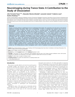
ABSTRACT
Epilepsy is one of the most important chronic neurological disorders worldwide affecting more
than 50 million people of all ages. Among these almost 20% of epilepsy cases are uncontrollable
and have an unknown source of this abnormal electrical activity.
The present methods for detection of the epileptogenic foci comprises positron emission
tomography, single photon emission computed tomography, magnetoencephalography,
electroencephalography (EEG) alone and EEG/functional magnetic resonance imaging (fMRI), all
with limitations in terms of temporal and spatial resolutions. In order to overcome some of those
limitation a new method using fMRI alone was developed based on the hypotheses that the
epileptogenic focus shows Blood Oxygen Level Dependent (BOLD) temporal profiles distinct
from the remaining brain parenchyma during interictal activity and that the epileptogenic focus
BOLD signals show lower complexity than healthy parenchyma.
Therefore, bi-dimensional temporal clustering analysis (2dTCA), a data-driven technique, was
used to identify brain regions with similar temporal profiles. Then, the BOLD signals of these
regions were assessed regarding complexity using a modified multiscale entropy algorithm and
also detrended fluctuation analysis in order to identify which of those regions corresponded to
epileptogenic tissue.
In order to demonstrate the applicability of the developed method a sample of three epileptic
patients were analyzed comprising three types of epilepsy: unilateral and bilateral temporal lobe
epilepsies, and focal cortical dysplasia. The results showed that this method is able to detect the
brain regions associated with epileptogenic tissue. The results also showed that the
epileptogenic focus influences the dynamics of related brain networks. This could be a key factor
in the applicability of this method to other epilepsy cases.
Finally, new perspectives are envisioned concerning the use of this method in the medical care
of epilepsy and in the study of other brain networks.
KEYWORDS
Epilepsy; epileptogenic focus; functional magnetic resonance imaging; temporal clustering
analysis; complexity analysis.
vii
CONTENTS
Acknowledgments .......................................................................................................................... i
Resumo......................................................................................................................................... iii
Palavras-Chave ..............................................................................................................................vi
Abstract ........................................................................................................................................vii
Keywords ......................................................................................................................................vii
List of Figures ................................................................................................................................xi
List of Tables ............................................................................................................................... xvii
List of Acronyms ........................................................................................................................ xviii
Chapter 1.
Introduction and Objectives .................................................................................. 1
1.1.
BOLD signal origin and fMRI analysis ............................................................................ 3
1.2.
Epileptogenic focus localization .................................................................................... 5
1.3.
Complexity analysis ....................................................................................................... 6
1.4.
Thesis hypotheses and goals ......................................................................................... 7
Chapter 2.
Bi-dimensional Temporal Clustering Analysis ....................................................... 9
2.1.
Introduction .................................................................................................................. 9
2.2.
Materials and Methods ............................................................................................... 13
2.2.1.
Simulated Dataset Characterization.................................................................... 13
2.2.2.
Algorithm implementation .................................................................................. 14
2.2.3.
Performance analysis of simulated dataset: sensitivity analysis ........................ 19
2.3.
Results ......................................................................................................................... 20
2.4.
Discussion .................................................................................................................... 21
Chapter 3.
Multiscale Entropy .............................................................................................. 23
3.1.
Introduction ................................................................................................................ 23
3.2.
Materials and Methods ............................................................................................... 25
3.2.1.
Modified MSE: Algorithm implementation ......................................................... 26
viii
3.2.2.
Illustrative examples ........................................................................................... 29
3.3.
Results ......................................................................................................................... 31
3.4.
Discussion .................................................................................................................... 34
Chapter 4.
Detrended Fluctuation Analysis .......................................................................... 36
4.1.
Introduction ................................................................................................................ 36
4.2.
Materials and Methods ............................................................................................... 38
4.2.1.
4.2.2.
Algorithm implementation .................................................................................. 38
Illustrative examples ............................................................................................... 41
4.3.
Results ......................................................................................................................... 41
4.4.
Discussion .................................................................................................................... 44
Chapter 5.
5.1.
Epileptic Patients Study ....................................................................................... 46
Introduction ................................................................................................................ 46
5.1.1.
Types of epilepsy ................................................................................................. 46
5.1.2.
Epileptic activity and its influence on functional brain connectivity .................. 46
5.1.3.
Revisiting methodological hypotheses................................................................ 47
5.2.
Materials and Methods ............................................................................................... 48
5.2.1.
Sample characterization ...................................................................................... 48
5.2.2.
Pipeline Analysis .................................................................................................. 48
5.3.
Results ......................................................................................................................... 53
5.3.1.
Patient 1 – Unilateral Temporal Lobe Epilepsy (TLE): left TLE ............................ 53
5.3.2.
Patient 2 – Bilateral TLE: with right temporo-parietal predominance ................ 58
5.3.3.
Patient 3 – Focal Cortical Dysplasia Epilepsy (FCDE): right precentral gyrus ...... 65
5.4.
Discussion .................................................................................................................... 71
5.4.1.
Patient 1 – Unilateral TLE: left TLE ...................................................................... 71
5.4.2.
Patient 2 – Bilateral TLE: with right temporo-parietal predominance ................ 72
5.4.3.
Patient 3 – FCDE: right precentral gyrus ............................................................. 72
5.4.4.
General Discussion .............................................................................................. 73
Closing remarks ........................................................................................................................... 76
ix
References................................................................................................................................... 77
Appendix A .................................................................................................................................. 86
Appendix B .................................................................................................................................. 88
Appendix C .................................................................................................................................. 89
x
LIST OF FIGURES
Fig. 1- Relative spatial and temporal sensitivities of different functional brain imaging methods.
MEG: magnetoencephalography; sEEG: scalp electroencephalography; fMRI: functional
magnetic resonance imaging; PET: positron emission tomography; SPECT: single photon
emission computed tomography. Adapted from (Jezzard et al. 2001)......................................... 2
Fig. 2- BOLD Signal Response to a brief stimulus. Adapted from (Jezzard 1999). ........................ 3
Fig. 3- Steps involved in the processing of fMRI data. Adapted from (Clare 1997). ..................... 4
Fig. 4- Results from an epileptic patient with unknown focus localization. a: activation map of
peaks determined with TCA; b: histogram output from TCA; c: response of the voxel indicated
by the arrow (dotted line) with modeled BOLD response time course (solid line). Adapted from
(Morgan et al. 2004)...................................................................................................................... 9
Fig. 5- Statistical maps from a subject with epilepsy obtained with models derived from TCA and
from EEG. Adapted from (Hamandi et al. 2005). ........................................................................ 10
Fig. 6- Graphical depiction of the TCA and 2dTCA algorithms showing how multiple reference
time courses are created by the 2dTCA algorithm when multiple different voxel time courses are
present in the data (Morgan et al. 2008). x represents the time point at which the voxel’s time
series is maximum. y represents the time point at which occurs a significant signal increase on
the time series. ............................................................................................................................ 12
Fig. 7- Depiction of the two regions in which the epileptic activity was simulated. A) 216 voxels
cubic regions located at the left temporal lobe. B) 216 voxels cubic regions located at right
frontal lobe. In each frame, A) and B), the top left, top right, and bottom left images represent
a sagittal, coronal and transverse view, respectively. ................................................................ 13
Fig. 8- BOLD signal created by the convolution of the HRF with a spike train containing the timing
of each event (Top) and its addition to the BOLD signal already presented in the real data
(Bottom). ..................................................................................................................................... 14
Fig. 9- Example of the three baselines (one corresponding to the mean of each cluster) estimated
from k-means technique. The scale at the right represents the percentage signal change
computed with the baseline corresponding to the mean of the middle cluster. ....................... 15
Fig. 10- Average sensitivity/specificity analysis for thresholds definition of candidate voxels
selection step. Keeping the average sensitivity above 90 %, the best average specificity (red
circle) was found for up and low boundaries of 3 and 0.5%, respectively, and a threshold of 2
standard deviations above the baseline with a TPR equal to 0.98 and a correspondent FPR equal
to 0.59. The area under the curve is equal to 0.62. .................................................................... 16
xi
Fig. 11- Illustration of the second step of grouping RTCs. It is based on the percentage of shared
activity between two RTCs. A: Temporal profile of two hypothetic RTCs. B: binary representation
of each RTC spike above the mean, where the white color represents activations. .................. 18
Fig. 12- Average sensitivity/#RTCs analysis for correlation coefficient (Top) and shared activity
(Bottom) threshold definition of RTC grouping step. Optimal parameters for correlation
coefficient and shared activity threshold were both defined as 0.7 with a correspondent average
TPR and FPR and an average of RTCs number of 0.52, 0.0632 and 18.8 for the first threshold and
0.518, 0.0628 and 18.9 for the second threshold, respectively. ................................................ 19
Fig. 13- TPR (left column)/FPR (right column) analysis on simulated data among ROIs size and
HRF amplitude above the baseline. Top row: simulated epileptic activity with 5 spikes. Bottom
row: simulated epileptic activity with 10 spikes. ........................................................................ 20
Fig. 14- Schematic illustration of the coarse-graining procedure (Costa et al. 2005). ................ 23
Fig. 15- Top: Simulated white and 1/f noises. Bottom: MSE analysis of simulated white and 1/f
noise time series. Adapted from (Costa et al. 2005). .................................................................. 24
Fig. 16- Schematic illustration of the modified coarse-graining procedure where a moving
average is applied to the original time-series for each scale factor. Adapted from (Costa et al.
2005). .......................................................................................................................................... 26
Fig. 17- Illustration of sample entropy computation. In this example, the pattern length m and
the tolerance r are 2 and 20, respectively. Dotted horizontal lines around data points u[1], u[2]
and u[3] represent u[1] ± r, u[2] ± r, and u[3] ± r, respectively. All green, red, and blue, points
represent data points that match the data point u[1], u[2], and u[3], respectively. Adapted from
(Costa et al. 2005). ...................................................................................................................... 27
Fig. 18- Scoring classification for each possible pair of parameters (pattern length - m, tolerance
- r) with a tested m = 2 (light blue) and 3 (dark blue) and r = 0.1 to 0.5 in steps of 0.05. Each bar
represents the total score attributed to that case. The results showed that the optimal values
for m and r are 3 and 0.4 times the standard deviation, respectively, with a total score of 67. 28
Fig. 19- Top: Sinusoidal time series with a frequency and sample frequency of 0.01 Hz and 0.5
Hz, respectively, and a length of 250 time points. Bottom: 1/f2 noise time series with a length of
250 time points. .......................................................................................................................... 30
Fig. 20- Sample entropy profile (computed with m=3 and r=0.4) over scale for original time series
of white (asterisk) and 1/f (circle) noises of length 1000 time points using the original (blue) and
the modified (red) MSE algorithm. ............................................................................................. 31
Fig. 21- Left: Sample entropy profile (computed with m=3 and r=0.4) over scale for original time
series of white (asterisk) and 1/f (circle) noises with lengths in the range of 100 to 250 time
points, in increments of 50, using the original (Top) and the modified (Bottom) MSE algorithm.
xii
Right: CI distribution in function of time series length correspondent to the sample entropy
analysis presented at left. ........................................................................................................... 32
Fig. 22- Left: Sample entropy profile (computed with m=3 and r=0.4) over scale for time series
of white (in blue), 1/f (in red) and 1/f2 (in green) noises, and sinusoidal signals of 0.01 Hz (in cyan)
and 0.1 Hz (in black) with a length of 250 time points using the modified MSE algorithm. Right:
Corresponding CI values for each signal type presented at left. CIWhite noise = 17.2; CI1/f noise = 8.1;
CI1/f2 noise = 3.8; CIsinusoid 0.01 Hz = 3.2; CIsinusoid 0.1 Hz = 0 ..................................................................... 33
Fig. 23- Illustration of DFA algorithm steps. For this example a 1/f noise time series was created
with a length of 1000 time points. The steps A to E represents the procedure for a window
length, Nw, of 100 data points. F represents the final output when the previous steps were
repeated for all Nw values. : scaling exponent; F: RMS fluctuation. ......................................... 39
Fig. 24- Scoring classification for each possible pair of parameters (maximum percentage - pmax,
overlap) with a tested range 50 % (dark blue), 40 % (light blue), 30 % (white), 20 % (gray), and
10 % (black) for pmax and 0 to 50 % in steps of 10 % for the overlap. Each bar represents the total
score attributed to that case. The results showed that the optimal values for pmax and overlap
are both 40 % with a total score of 117. ..................................................................................... 40
Fig. 25- Double logarithmic plot of fluctuations (computed with pmax and overlap equal to 40 %)
over window length for white (asterisk) and 1/f (circle) noise time series of length 1000 time
points using the DFA algorithm. The fitting line for each fluctuations profile is represented at red
for white and at blue for 1/f noises. ........................................................................................... 42
Fig. 26- Left:  value (computed with pmax and overlap equal to 40 %) for time series of white
(asterisk) and 1/f (circle) noise with lengths of the time series in the range of 100 to 250 time
points, in increments of 50, using the DFA algorithm. Right: AI distribution in function of time
series length correspondent to the  values presented at the left. ........................................... 43
Fig. 27- Left: Double logarithmic plot of fluctuations (computed with pmax and overlap equal to
40 %) over window length for time series of white (in blue), 1/f (in red) and 1/f2 (in green) noises,
and sinusoidal signal of 0.01 Hz (in cyan) and 0.1 Hz (in black) with a length of 250 time points
using DFA algorithm. Right: Corresponding  values for each signal type presented at left. White
noise
= 0.52; 1/f noise = 0.94; 1/f2 noise = 1.3; sinusoid 0.01 Hz = 1.6; sinusoid 0.1 Hz = 0.093. .................... 43
Fig. 28- Influence of sample frequency and sinusoidal frequency (in Hz) on  value. ............... 44
Fig. 29- Flowchart illustrating the pipeline analysis of real subject data, namely, epileptic
patients’ dataset. : scaling exponent; AI: Anisotropy index; CI: Complex Index; DFA: Detrended
Fluctuation Analysis; GLM: General Linear Model; FEWR: Family-Wise Error Rate; k: extended
threshold; MSE: Multiscale Entropy; RTC: Reference Time Course; SPM: Statistical Parametric
xiii
Map. Circles on CI/ distribution: blue: white noise; red: 1/f noise; green: 1/f2 noise; cyan:
sinusoid of 0.01 Hz; black: sinusoid of 0.1 Hz. ............................................................................ 49
Fig. 30- Histogram showing the distribution of the number of voxels with a given value of the
transient spike selection limit [2 standard deviations (std) above the baseline] for patient 1. Red
dashed lines represents the lower and upper boundaries of allowed signal change (see Chapter
2: 2.2.2 Algorithm implementation – Candidate voxels selection). ............................................ 53
Fig. 31- Results for patient 1. Left: bi-dimensional histogram with the counting of transient spikes
over the time. Each column represents a preliminary RTC. Right diagonal profile representing
the number of voxels which maximum occurs in each time point. ............................................ 54
Fig. 32- Activation maps from RTC_1, RTC_5, RTC_7 and RTC_15 obtained using 2dTCA (FEWR
correction, p-value<0.05, k-threshold=27 voxels) and corresponding RTCs’ temporal profiles.
Results for patient 1. S: superior; I: inferior; A: anterior; P: posterior; R: right; L: left. .............. 55
Fig. 33- Correlation matrix between ipsi and contralteral clusters of all RTCs that produced SPMs
with significant activation. Results for patient 1. Each label on the left of the matrix as the form
of ‘Idx: RTC#_size’ or ‘Idx: RTC#_size_c’, where Idx represents the index of the label, # the
number of the RTC that produced the SPM, size stands for the size of the cluster being analyzed,
and c means contralateral cluster. On the bottom of the matrix are the labels with the same
indexes as those presented on the left. ...................................................................................... 56
Fig. 34- Distribution of the mean CI and  across each cluster of RTC 5 and the CI and  for the
ipsi and lateral cluster of RTC 7. At blue are the mean parameters for ipsilateral clusters and at
red are the mean parameters for contralateral clusters. Results for patient 1.......................... 56
Fig. 35- Anisotropy analysis of each cluster considered for further analysis. At green is the target
region. Each red point is labeled in the following way: ‘Number of the RTC’-‘Size of the RTC’.
Results for patient 1. ................................................................................................................... 57
Fig. 36- CI/ distribution of each cluster considered for further analysis. Each red point is labeled
in the following way: ‘Number of the RTC’-‘Size of the RTC’. Results for patient 1. .................. 58
Fig. 37- Functional connectivity maps of RTC5_30 (the potential epileptogenic focus chosen by
complexity analysis) in z-score and thresholded at ±0.51. Results for patient 1. L: left; R: right.
..................................................................................................................................................... 58
Fig. 38- Histogram showing the distribution of the number of voxels with a given value of the
transient spike selection limit [2 standard deviations (std) above the baseline] for patient 2. Red
dashed lines represents the lower and upper boundaries of allowed signal change (see Chapter
2: 2.2.2 Algorithm implementation – Candidate voxels selection). ............................................ 59
xiv
Fig. 39- Results for patient 2. Left: bi-dimensional histogram with the counting of transient spikes
over the time. Each column represents a preliminary RTC. Right diagonal profile representing
the number of voxels which maximum occurs in each time point. ............................................ 59
Fig. 40- Activation maps from RTC_1, RTC_2, RTC_3, RTC_5, RTC_10, and RTC_14 obtained using
2dTCA (FEWR correction, p-value<0.05, k-threshold=27 voxels) and corresponding RTCs’
temporal profiles. Results for patient 2. S: superior; I: inferior; A: anterior; P: posterior; R: right;
L: left............................................................................................................................................ 61
Fig. 41- Correlation matrix between ipsi and contralteral clusters of all RTCs that produced SPM
with significant activation. Results for patient 2. Each label on the left of the matrix as the form
of ‘Idx: RTC#_size’ or ‘Idx: RTC#_size_c’, where Idx represents the index of the label, # the
number of the RTC that produced the SPM, size stands for the size of the cluster being analyzed,
and c means contralateral cluster. On the bottom of the matrix are the labels with the same
indexes as those presented on the left. ...................................................................................... 62
Fig. 42- Distribution of the mean CI and  across each cluster of RTC_3, RTC_5, RTC_10, and
RTC_14 and the CI and for the ipsi and contralateral cluster of RTC_2. At blue are the mean
parameters for ipsilateral clusters and at red are the mean parameters for contralateral clusters.
Results for patient 2. ................................................................................................................... 63
Fig. 43- Anisotropy analysis of each cluster considered for further analysis. At green is the target
region. Each red point is labeled in the following way: ‘Number of the RTC’-‘Size of the RTC’.
Results for patient 2. ................................................................................................................... 63
Fig. 44- CI/ distribution of each cluster considered for further analysis. Each red point is labeled
in the following way: ‘Number of the RTC’-‘Size of the RTC’. Results for patient 2. .................. 64
Fig. 45- Functional connectivity maps of RTC10_92 (the potential epileptogenic focus chosen by
complexity analysis) in z-score and thresholded at ±0.4. Results for patient 2. L: left; R: right. 65
Fig. 46- Histogram showing the distribution of the number of voxels with a given value of the
transient spike selection limit [2 standard deviations (std) above the baseline] for patient 3. Red
dashed lines represents the lower and upper boundaries of allowed signal change (see Chapter
2: 2.2.2 Algorithm implementation – Candidate voxels selection). ............................................ 65
Fig. 47- Results for patient 3. Left: bi-dimensional histogram with the counting of transient spikes
over the time. Each column represents a preliminary RTC. Right diagonal profile representing
the number of voxels which maximum occurs in each time point. ............................................ 66
Fig. 48- Activation maps from RTC_1, RTC_3, RTC_4 and RTC_11 obtained using 2dTCA (FEWR
correction, p-value<0.05, k-threshold=27 voxels) and corresponding RTCs’ temporal profiles.
Results for patient 3. S: superior; I: inferior; A: anterior; P: posterior; R: right; L: left. .............. 67
xv
Fig. 49- Correlation matrix between ipsi and contralteral clusters of all RTCs that produced SPM
with significant activation. Results for patient 3. Each label on the left of the matrix as the form
of ‘Idx: RTC#_size’ or ‘Idx: RTC#_size_c’, where Idx represents the index of the label, # the
number of the RTC that produced the SPM, size stands for the size of the cluster being analyzed,
and c means contralateral cluster. On the bottom of the matrix are the labels with the same
indexes as those presented on the left. ...................................................................................... 68
Fig. 50- Distribution of the mean CI and  across each cluster of RTCs 1, 3, 4, and 11. At blue are
the mean parameters for ipsilateral clusters and at red are the mean parameters for
contralateral clusters. Results for patient 3. ............................................................................... 69
Fig. 51- Anisotropy analysis of each cluster considered for further analysis. At green is the target
region. Each red point is labeled in the following way: ‘Number of the RTC’-‘Size of the RTC’.
Results for patient 3. ................................................................................................................... 69
Fig. 52- CI/ distribution of each cluster considered for further analysis. Each red point is labeled
in the following way: ‘Number of the RTC’-‘Size of the RTC’. Result for patient 3. .................... 70
Fig. 53- Functional connectivity maps of RTC11_39 (the potential epileptogenic focus chosen by
complexity analysis) and RTC4_55 (the cluster that best described the anatomical brain region
with lesion) in z-score and thresholded at ±0.36 and ±0.46, respectively. Results for patient 3. L:
left; R: right.................................................................................................................................. 70
xvi
LIST OF TABLES
Table 1- Epileptic patients sample characterization: gender, age, type of epilepsy, and
localization of its epileptogenic focus. F: female; M: male; TLE: temporal lobe epilepsy; FCDE:
focal cortical dysplasia epilepsy. ................................................................................................. 48
Table 2- Number and size of the clusters presented in each SPM of patient 1. ......................... 54
Table 3- Number and size of the clusters presented in each SPM of patient23. ........................ 60
Table 4- Number and size of the clusters presented in each SPM of patient 3. ......................... 66
xvii
LIST OF ACRONYMS
2dTCA

Two-dimensional Temporal Clustering Analysis

Scaling Exponent
AI
Anisotropy Index
BOLD
Blood Oxygen Level Dependent
CI
Complexity Index
dHb
Deoxyhemoglobin
EEG
Electroencephalography
EPI
Echo Planar Imaging
FDG
Fluorodeoxyglucose
fMRI
Functional Magnetic Resonance Imaging
FWER
Family-Wise Error Rate
DFA
Detrended Fluctuation Analysis
DMN
Default Mode Network
GLM
General Linear Model
HRF
Hemodynamic Response Function
ICA
Independent Component Analysis
iEEG
Intracranial Electroencephalography
LRTC
Long-Range Temporal Correlations
MEG
Magnetocencephalography
MSE
Multiscale Entropy Analysis
oHb
Oxyhemoglobin
PET
Positron Emission Tomography
RMS
Root-Mean-Square
ROI
Region-of-Interest
RTC
Reference Time Course
xviii
sEEG
Scalp Electroencephalography
SPM
Statistical Parametric Map
SNR
Signal-to-Noise Ratio
TCA
Temporal Clustering Analysis
xix
CHAPTER 1. INTRODUCTION AND OBJECTIVES
Epilepsy is one of the most important chronic neurological disorders worldwide affecting more than
50 million people of all ages. Although 70% of the cases are treatable with anti-epileptic drugs and
less than 10% with surgical therapy, the remaining 20% can’t control their seizures. This neurological
disorder brings an important impact on epileptic patients concerning discrimination, social stigma,
and higher national healthcare costs. People with epilepsy can be targets of prejudice and the stigma
of the disorder can discourage people from seeking treatment for symptoms and becoming
identified with the disorder (WHO 2012).
An epileptic seizure can be defined as a “transient occurrence of signs and/or symptoms due to
abnormal excessive or synchronous neuronal activity in the brain” (Fisher et al. 2005). These brief
electrical disturbances can have effects on sensory, motor, and autonomic functions, provoke
changes in awareness or behavior, loss of consciousness, and convulsions. Uncontrolled epilepsy
can also lead to depression, anxiety, and loss of cognitive function (Avanzini et al. 2013).
The epileptogenic zone or focus is a theoretical concept corresponding to the brain volume that
needs to be removed to render the patients seizure-free, i.e., it describes the abnormal cortex
responsible for the generation of epileptic seizures. Thus, the cessation of seizures is accomplished
with the complete resection of this area (Hamandi et al. 2005). This focus is characterized by two
types of electrical activity, ictal which means during seizure, and interictal, which mean between
seizures. The last one is normally more brief in time and is periodic (Ko et al. 2014).
Hereupon, epileptogenic focus identification is important to epilepsy diagnostic and seizure control.
The present methods for this purpose are based on Positron Emission Tomography (PET) and Single
Photon Emission Computed Tomography (SPECT) (Mountz 2007; Kim & Mountz 2011),
Magnetoencephalography (MEG) (Foley et al. 2014), Electroencephalography (EEG) alone
(Hassanpour et al. 2004; Leal et al. 2007; Leal et al. 2008) and EEG/functional Magnetic Resonance
Imaging (fMRI) analysis (Leal et al. 2006; Leite et al. 2013; Wang et al. 2012; Hamandi et al. 2005;
Thornton et al. 2010). There’s a tradeoff in terms of time and spatial resolutions for all these
techniques (Fig. 1). The first technique is a direct measure of the Fluorodeoxyglucose (FDG) uptake
in the brain based on the hypotheses that the cortical blood flow increases in the area of seizure
1
discharge (Mountz 2007). The second
one works is a similar way, but with a
MEG/
SPECT
different radiotracer (Tc-99m) (Kim &
Mountz 2011). The main limitation of
using PET and SPECT to localize the
epileptogenic zone relies on specificity
of abnormalities due to its limited
spatial resolution and poor temporal Fig. 1- Relative spatial and temporal sensitivities of different functional
resolution (Morgan et al. 2004; Clare brain imaging methods. MEG: magnetoencephalography; sEEG: scalp
1997). Furthermore, the need for a
radiotracer is also a drawback, making
electroencephalography; fMRI: functional magnetic resonance
imaging; PET: positron emission tomography; SPECT: single photon
emission computed tomography. Adapted from (Jezzard et al. 2001).
this technique more invasive.
The third and fourth techniques used to localize ictal and interictal electrical activity are MEG and
EEG. There are two main modes of using the latter modality, scalp EEG (sEEG) and intracranial EEG
(iEEG). Both of these modalities have high temporal resolution, allowing the detection of brief spikes
of electric activity, such as interictal activity. However, when regarding the needs of abnormalities’
specificity for presurgical assessment, the spatial resolution of sEEG and MEG is poor. In order to
improve the resolution of sEEG a high-density of electrodes is needed (Leal et al. 2007; Leal et al.
2008). This issue can be overcome by iEEG, as the electrical signal is recorded directly from cortical
tissue. The major drawback of this last modality relies on the fact that it’s extremely invasive.
Lastly, simultaneous EEG-fMRI is an emergent technique which combines the best of two modalities,
high temporal resolution from EEG and high spatial resolution from fMRI. The strategy followed in
this case is to continuously sample the interictal and ictal events while measuring the BOLD signal
simultaneously with EEG. This is somewhat cumbersome as it requires a very specific and delicate
setup, particularly for acceptable recording of the EEG. Otherwise it will bring several kinds of noise
problems, including movements artifacts (Wang et al. 2012), compromising the feasibility of EEGfMRI studies. Another shortcoming associated with this technique, and with EEG alone, is that they
aren’t sensitive to interictal epileptiform activity in deep structures making this technique useful
only in patients with frequent interictal events recorded from the sEEG (Morgan et al. 2004; Lopes
et al. 2012). To overcome some of the limitations described above and find a more suitable solution
to localize a seizure onset, efforts are being taken to develop new processing methods using fMRI
2
technique only (Yee & Gao 2002; Morgan et al. 2004; Hamandi et al. 2005; Morgan et al. 2008;
Morgan et al. 2010).
Another approach to epilepsy diagnosis and characterization of epileptic signals behavior has been
recently taken on the complexity field. Some authors have been hypothesized that epileptogenic
brain tissue has a different complexity than healthy brain tissue (Parish et al. 2004; Monto et al.
2007; Protzner et al. 2010). A complete characterization of this complexity could lead to a definition
of a physiological biomarker applicable to epilepsy, namely for diagnostic and monitoring of its
treatment. For that purpose two main approaches can be used: a disorder level based (Ouyang et
al. 2009; Protzner et al. 2010) or a fractal properties based (Parish et al. 2004; Monto et al. 2007)
methods. In both of them it is expected that in the epileptogenic focus the complexity is lower
because of its intrinsic periodic interictal electric activity.
This thesis project will focus on the epileptic focus localization through fMRI BOLD signals and then
on the complexity analysis of its time series. Therefore, in the next section the concepts inherent to
this work will be described.
1.1. BOLD signal origin and fMRI analysis
Functional magnetic resonance imaging (fMRI) is a powerful non-invasive tool that allows the study
of the functional responses of the brain in a quantitative way. One advantage of using fMRI is the
identification of brain activity due to a stimulus with a high spatial resolution (Jezzard et al. 2001).
This technique is based on the
hemodynamic response function
(HRF) of the brain, which arises
B
when a given stimulus is applied.
The HRF is a transfer function of
the
neurovascular
coupling
A
characteristic of brain activation.
When a stimulus acts on a
C
particular region of the brain
evokes, in that area, a change in
blood
flow.
This
Fig. 2- BOLD Signal Response to a brief stimulus. Adapted from (Jezzard
facilitates 1999).
3
glucose oxidation by providing more oxygen molecules. If there is an increased consumption of
oxygen, there’ll be an increased concentration of deoxyhemoglobin (dHb), a paramagnetic oxygen
binding molecule. Oxyhemoglobin (oHb), on the other hand, is a diamagnetic molecule with a
magnetic susceptibility smaller than that of dHB (Clare 1997).
Therefore, a change in hemoglobin oxygenation leads to changes in the local distortions of a
magnetic field applied, generating local field gradients and local changes of T2* in tissue the blood
vessels. The measure of the T2* originate the BOLD signals (Jezzard et al. 2001), see Fig. 2. The brain
hemodynamic response can be summarized in the following steps. When a brief stimulus acts,
there’s an initial decrease of BOLD signal due to increase of oxygen consumption (Fig. 2A). Then, the
increased blood flow decreases the dHb concentration increasing the BOLD signal (Fig. 2B). Finally,
a delay of the return to the initial blood volume level provokes a decrease of oHb, and a
consequently increase of dHb reducing temporally the BOLD signal intensity (Fig. 2C).
The output of fMRI is a set of volumes comprising the scans of
the brain at successive times, usually named raw data. Each
Raw Data
volume is divided in resolution dependent number of small
elements, named voxels, in which the information of the
correspondent brain region is stored. One of the goals of
Pre-processing
acquiring fMRI data is to perform a robust, sensitive, and valid
analysis to detect brain regions that show increased signal
Statistical analysis
intensity at the stimulus time. In other words, the aim of fMRI
analysis is to identify which voxels have their signal
significantly greater than the noise level (Clare 1997; Jezzard
Inference and
Presentation
et al. 2001). A typical pipeline analysis, schematically
represented in Fig. 3, includes a first step of raw data pre-
Fig. 3- Steps involved in the processing of
fMRI data. Adapted from (Clare 1997).
processing that usually includes, correction to time effects and
to subject movement during the experiment, and data spatial smoothing to improve the signal to
noise ratio. Additional steps, such as, data detrending, filtering and regressing out of nuisance
covariates are often taken. The aim of this pre-process is to improve the detection of activation
events. Then, a statistical analysis is performed to detect which voxels shows a response to the
assessed stimulus. This step usually involves a model estimation, through a general linear model
(GLM) based on convolution between the HRF and the stimulus temporal profile. Finally, in order to
display the activation images, statistical confidence must be given to the results by inferring about
4
probability values. See Appendix A for more information about statistical analysis, inference and
statistical maps presentation in fMRI.
The assessment of a stimulus via a pipeline analysis as described above can be one of two types.
The first one comprises a stimulus that has typically few time points of duration, and its analysis is
usually named a block-related one. The second one, a transient stimulus with a short duration is
used, whereby its analysis is named an event-related one (Josephs et al. 1997). In epilepsy, once the
stimulus is usually a transient spike corresponding to interictal electric activity, the analysis
described in the above pipeline of event-related type.
Since no technique is free of shortcomings this one has several limitations too. One of them
concerns the temporal resolution, which is limited by the profile of the hemodynamic response, and
low signal-to-noise ratio (SNR) and contrast-to-noise ratio (CNR), leading to high variance in the
results. One way to overcome this last limitation is to repeat the stimuli more than once, decreasing
variance in results (Jezzard et al. 2001). However, this is difficult to apply in epilepsy since the timing
of the stimulus, interictal or ictal seizure activity, is random and uncontrollable (Morgan et al. 2007).
1.2. Epileptogenic focus localization
As explained before, the timing of ictal and interictal activity in epilepsy is unknown and
unpredictable. Therefore, an analysis based on models isn’t suitable to localizing the epileptogenic
focus, since no assumptions about temporal profile of the stimuli can be made. Data-driven
techniques have been developed to deal with such cases as they are model-free. Some examples of
such methods are the following: principal component analysis (Sugiura et al. 2004; You et al. 2011),
independent component analysis (ICA) (Rodionov et al. 2007), hierarchical clustering (Cordes et al.
2002; Keogh et al. 2005), and fuzzy clustering (Somorjai & Jarmasz 2003; Wahlberg & Lantz 2000).
When applied to fMRI datasets these methods result in a large number of components, which are
hard to classify without spatial and temporal information (De Martino et al. 2007; Rodionov et al.
2007).
Another data-driven method developed in the past years is temporal clustering analysis (TCA) (Yee
& Gao 2002; Gao & Yee 2003; Morgan et al. 2004; Hamandi et al. 2005). This is a one-dimensional
algorithm that groups together time series to one single cluster with the same temporal profile
based on a given criteria. This criterial could be, for example, the same maximum signal magnitude
5
timing or the same first signal magnitude increase, to one single cluster. A modification of the
original TCA to a bi-dimensional method, two-dimensional temporal clustering analysis (2dTCA)
(Morgan et al. 2007; Morgan et al. 2008), detects different BOLD responses, assumed to be from
different sources. It allows the detection of more than one single cluster. Once obtained the
temporal profile of the cluster, it is possible to perform an event-related fMRI analysis.
In Morgan’s work (Morgan et al. 2007; Victoria L Morgan et al. 2008; Morgan et al. 2010) the
application of 2dTCA to epileptogenic focus localization is based on the hypothesis that interictal
epileptic activity provokes a transient BOLD spike with a rate slower than that of BOLD images
acquisition. This hypothesis was based on preview results of EEG-fMRI studies applied to temporal
lobe epilepsy (Salek-Haddadi et al. 2006; Kobayashi et al. 2005; Federico et al. 2005; Bagshaw et al.
2004). The main results of these works showed that interictal activity detected by EEG is associated
with a BOLD signal change.
1.3. Complexity analysis
The human brain has an inherent high complexity arising from the interaction of thousands of
neuronal networks that operates over a wide range of temporal and spatial scales (Hutchison et al.
2013). This enables the brain to adapt to the constantly changing environment and to perform
mental functions. In pathologic brains this capacity of adaptation is often impaired, leading to
ordered or random patterns of behavior. In case of epilepsy, the study of such complexity could help
to understand how an epileptic brain functions.
To assess brain complexity we can only observe the macroscopic output of brain function, such as
via EEG and fMRI, where a signal change represents a response from millions of neurons, thus
creating the need for robust methods to evaluate the complexity of signal from such techniques.
These methods are usually based on one of two approaches: disorder level based or a fractal
properties based.
The first one comprises methods that are entropy-based, by quantifying the regularity or orderliness
of a time series (Pincus 1991; Kurths et al. 1996; Andino et al. 2000; Richman & Moorman 2000).
Entropy can be conceptualized has a measure of the degree of disorder of a given system and
increases with the degree of irregularity, reaching its maximum in completely random systems, such
as uncorrelated or white noise, and its minimum in completely ordered systems, such as a single
6
frequency sinusoid. Physiologic outputs usually exhibits a higher degree of entropy under healthy
conditions than in a pathological state, as they’re characterized by a sustained breakdown of longrange correlations and loss of information (Goldberger et al. 2002). However, an increase in the
entropy may not always be associated with an increase in dynamical complexity (Costa et al. 2002).
One method that has been developed and improved in the past years and has been shown to
effectively quantify the complex dynamics of biological signals is the multiscale entropy (MSE) (Costa
et al. 2002). It is based on measuring the entropy over multiple time scales inherent in a time series.
The second approach on brain complexity assessment relies on the evaluation of long-range
temporal correlations (LRTC), which reflect the self-affinity of a given signal. The majority of
quantifications methods such as spectral analysis and Hurst analysis (Peng et al. 1995) for the LRTC
study are invalid to evaluate biological signals because, as they are complex and show fractal
properties, their stationarity are not guarantee. Thus, a method capable of detecting the LRTC was
developed in the past years to overcame the nonstationary problem of biological signals, named
detrended fluctuation analysis (DFA) (Peng et al. 1994).
1.4. Thesis hypotheses and goals
This master thesis project is based on the hypotheses that the epileptogenic focus shows a BOLD
signal with a distinct temporal profile from the remaining brain parenchyma, either during ictal and
interictal activity (Morgan et al. 2007; Victoria L Morgan et al. 2008; Morgan et al. 2010). Particularly,
it is known that the interictal epileptic activity provokes a transient BOLD spike with a rate slower
than that of BOLD images acquisition (Salek-Haddadi et al. 2006; Kobayashi et al. 2005; Federico et
al. 2005; Bagshaw et al. 2004). This makes possible the application of a method for the localization
of the epileptogenic focus, the 2dTCA.
Furthermore, it is well-known, from epileptic EEG signal studies, the periodic behavior of epileptic
activity of epileptogenic brain regions (Parish et al. 2004; Monto et al. 2007; Protzner et al. 2010).
Indeed, in these EEG studies it was shown that the epileptogenic focus EEG signal shows lower
complexity than healthy parenchyma. However, there are no studies showing the same results with
epileptic BOLD signals. Therefore, for the purpose of this thesis project it is hypothesized that the
epileptogenic focus BOLD signals shows lower complexity than healthy parenchyma. Also, this
complexity can be assessed by methods like MSE and DFA.
7
Summarizing, the innovation of this work is to explore the complexity properties of epileptic BOLD
signals through the application of an algorithm that localizes the epileptogenic focus and extracts
its BOLD signal. The main aim is to provide a definition of a biomarker for epileptic tissue
identification in order to help on the diagnostic, monitoring and treatment of epilepsy.
Hereupon, this thesis project have three main goals. First, the algorithms referred above, the 2dTCA,
the MSE, and the DFA, will be implemented in Matlab®1 language using the commercial software
package Matlab® R2014a. All of these methods will be optimized for BOLD signals analysis using
simulated data. Second, a study with a sample of epileptic patients will be carried out by first
localizing potential epileptogenic foci with 2dTCA and analyzing complexity of its BOLD signal in
order to compare with those of healthy brain parenchyma. Third, based on the hypotheses stated
above, the most likely epileptogenic focus will be chosen.
1
The MathWorks Inc., Natick, MA, 2000 (http://www.mathworks.com/)
8
CHAPTER 2. BI-DIMENSIONAL TEMPORAL CLUSTERING ANALYSIS
2.1. Introduction
TCA was firstly introduced by Liu and colleagues with a pioneer work where this method was used
to study the temporal response of the brain after eating (Liu et al. 2000). The problem addressed by
this approach was the fact that there’s no model assumption that can be taken to estimate which
brain regions will be activated after eating, once the activation timing is unknown. This algorithm
searches for the maximal response in each voxel’s time series converting a four-dimensional data,
characterized in terms of space and time, into a simple relationship between the number of voxels
reaching maximum signals and the time, named histogram. A concept of brain parcellation that
accounts for timing and connectivity was accomplished for the first time with the results of this
work.
In order to improve the brain
activations timing detection Yee
and Gao modified the sensitivity
of TCA algorithm basing the
method on the integrated signal
intensity of a temporal cluster at
each time point (Yee & Gao 2002;
Gao & Yee 2003) rather than only
on the size of a temporal cluster
(Liu et al. 2000). In other words,
in the modified algorithm a
condition
is
superimposed
limiting the maximum signal
change allowed to be clustered.
The results of Yee and Gao work
show that, despite the fact that
the
modified
TCA
is
more
sensitive than the original one,
Fig. 4- Results from an epileptic patient with unknown focus localization. a:
activation map of peaks determined with TCA; b: histogram output from TCA;
c: response of the voxel indicated by the arrow (dotted line) with modeled
neither of them could detect BOLD response time course (solid line). Adapted from (Morgan et al. 2004).
9
peaks smaller than the noise level. This opened a window to novel problems, like time shift and
movement artifacts, that needed to be addressed before the TCA application.
The application of TCA to epileptogenic focus localization was first addressed by Morgan and
colleagues in (Morgan et al. 2004) under the hypothesis that the timing of interictal activity could
be determined using TCA on resting fMRI data. Then, activation maps created by event-related fMRI
analysis using the discovered discharges timings could be determined to show which brain regions
are presumably part of the epileptogenic focus. The result from an epileptic patient with unknown
focus localization is shown in Fig. 4. It shows the histogram output from the TCA (Fig. 4b), the results
of statistical analysis (Fig. 4a), and fitted and adjusted responses of one voxel pertaining to the found
cluster (Fig. 4c). The fact that the TCA defines one single histogram, i.e., one single cluster, implies
that voxels spatially distant may be grouped together (as seen in Fig. 4). Whether this detected
cluster temporal profile is a representation of the epileptogenic focus or instead a mixture of
sources can’t be assessed and, therefore, the effectiveness of TCA can’t be assessed as well.
Fig. 5- Statistical maps from a subject with epilepsy obtained with models derived from TCA and from EEG. Adapted from
(Hamandi et al. 2005).
Hamandi and colleagues assessed the TCA performance by implementing and evaluating it, as
described in (Morgan et al. 2004), using fMRI data acquired with simultaneous EEG in patients with
clearly defined focal epilepsy and frequent interictal discharges (Hamandi et al. 2005). They
demonstrated that the temporal clusters found were closely correlated with motion events, and not
interictal epileptic activity, refuting the validity of using these as onsets in statistical analysis. In
order to illustrate this issue, there’s a resultant statistical map from an epileptic patient is present
10
in Fig. 5. It represents the activated brain region found with models in which the onsets were derived
either from TCA and EEG. As it can be seen those regions does not match with each other, contrary
as expected, suggesting that there may be a confounding with motion events when performing TCA.
Hamandi et al. work brought new insights about the limitations of using TCA applied to epilepsy,
suggesting that in order to improve this methodology there is the need to primarily separate the
noise from the stimuli source and then compare the performance of TCA with other method such
as ICA, for example.
Morgan and colleagues posterior work (Morgan et al. 2007; Morgan et al. 2008) brought a new
approach to this area by modifying the TCA methodology and overcoming some of the shortcomings
described above. They developed a two-dimensional TCA technique addressing the problem of
motion and physiological noise by detecting and sorting out separate BOLD responses assumed to
be from different sources. This was based on the assumption that BOLD signal changes due to
spontaneous interictal activity may be relatively small compared to those of noise, motion, and
other activity and are expected to be only slightly slower than the rate of image acquisition (Morgan
et al. 2008). Furthermore, as the shape of this BOLD signal response is well known it allows the
application of the 2dTCA.
Briefly, in Fig. 6 is depicted a graphical representation of how 2dTCA works and a comparison with
TCA. The 2dTCA algorithm will construct a bi-dimensional histogram where columns represent
temporal clusters with different temporal profiles. The criterion of grouping time series to different
clusters is based on the first time point at which the first signal increase occur, instead of grouping
with maximum signal criteria (Liu et al. 2000; Yee & Gao 2002; Gao & Yee 2003; Morgan et al. 2004;
Hamandi et al. 2005). This assumes that different sources of activation will not have overlapping
timing of BOLD response at the beginning of the time series, which is not proven to be in that way.
Supposing that in a functional dataset there are four voxels’ time series with different temporal
profiles (Vox 1 to 4 in Fig. 6), using 2dTCA Vox 1 and 2 were grouped together in the same histogram
column, representing a reference time course of one cluster. On the other hand Vox 3 and 4 will be
are grouped together in another column, representing another and independent reference time
course of a different cluster. If, for example, one group of voxels represent an epileptogenic focus
and another a noising source, such as movement, this algorithm could rule out the latter by sorting
different sources in different clusters. If a TCA approach were taken, all the voxel’s time courses
would be grouped together leading to the identification of brain regions that aren’t related to
epileptogenic tissue, similar to what was described in (Hamandi et al. 2005), see Fig. 5.
11
y
x
Fig. 6- Graphical depiction of the TCA and 2dTCA algorithms showing how multiple reference time courses are created by
the 2dTCA algorithm when multiple different voxel time courses are present in the data (Morgan et al. 2008). x represents
the time point at which the voxel’s time series is maximum. y represents the time point at which occurs a significant signal
increase on the time series.
In Morgan and colleagues’ work (Victoria L Morgan et al. 2008), the performance of 2dTCA was
assessed, in terms of specificity and sensitivity, by comparing it with the performance of TCA and
ICA applied to the same simulated data, where a well-known activations were defined (Morgan et
al. 2008). The results showed that 2dTCA algorithm can detect more than one independent
reference time course, or equivalently more than one temporal cluster, more effectively than TCA,
but slightly less effectively than ICA. However, they argued that as the 2dTCA algorithm will cluster
only transient spikes, while decreasing sensitivity to signals of other temporal characteristics, the
large number of components determined with ICA would make it difficult to determine the
components of interest in vivo when the activation regions are not known. This confirms the
advantage of using the 2dTCA as a data-driven for identifying the epileptogenic focus.
12
recent work have demonstrated that this algorithm can also be used to detects clusters associated
with the default-mode network (DMN) (Morgan et al. 2007; Morgan et al. 2008; Morgan et al. 2010;
Pizarro et al. 2012) in healthy (Cauda et al. 2010; Fox et al. 2005)and epileptic subjects and with
specific regions, such as the visual, auditory, and motor cortices, through external stimuli with
known timing (Morgan & Gore 2009).
2.2. Materials and Methods
2.2.1. Simulated Dataset Characterization
A
<
<
<
<
B
<
<
<
<
SPM
mip
SPM
mip
57.6349,9]9]
[10.806,57.6349,
[10.806,
[-58.5323,
8.09453]
-28.805,8.09453]
[-58.5323,-28.805,
As a final remark about the application of 2dTCA on healthy subjects and epileptic patients, more
<
<
-3
-3
x 10 -3
x 10
x 10-3
x 10
<
<
3
3
3
3
2
2
2
2
1
1
1
1
0
0
0
0
Fig. 7- Depiction of the two regions in which the epileptic activity was simulated. A) 216 voxels cubic regions located at
the left temporal lobe. B) 216 voxels cubic regions located at right frontal lobe. In each frame, A) and B), the top left, top
right, and bottom left images represent a sagittal, coronal and transverse view, respectively.
A simulated dataset was created, according to the pipeline presented in (Khatamian et al. 2011),
from a preprocessed rest fMRI healthy subject scan (see Appendix B for more details of this subject
data acquisition) by adding simulated BOLD signals in order to create simulated epileptic activity.
For this purpose two regions of interest (ROI) were defined (see Fig. 7), one in the left temporal lobe
(LTL) and the other in the right frontal lobe (RFL), to which simulated epileptic activity was added.
BOLD signals representing this type of activity were created by convolving the HRF with a spike train
containing the timing of each event (see Fig. 8) and added to the BOLD signal already presented in
each ROI. The final goal was to obtain simulated data with all combinations of the following
characteristics: 5 and 10 spikes randomly distributed in time, correspondent to LTL and RFL ROIs,
respectively; simulated activation amplitudes of 0.5 to 2% in increments of 0.25%; and ROI’s size of
27, 64, 125, and 216 voxels. Within a ROI the activation frequency and amplitude is homogenous.
Each simulation was repeated two times resulting in a total of 56 simulated datasets.
13
Template Stimulus
a.u.
a.u.
a.u.
0.5
1
Template Stimulus
0
0.5
Template Stimulus
0.5
-0.5
00
-0.5
-0.5
0.5
1
50
100
150
200
250
0
50
100
150
200
250
0
50
100
150
200
250
1
0
300
0.5
0
300
0
300
Simulated BOLD signal
800
820
780
1
Simulated BOLD signal
0
a.u.
a.u.
%change
a.u.
820
800
820
2
7800
800 0
-2
0
780
250
0.5
1
0
300
Simulated BOLD signal
Percent Sinal Change Transformation
0.5
1
50
100
50
100
50
100
150
200
150
200
250
0
300
0.5
150
200
250
300
200
250
0
300
Time (s)
0
50
100
150
Fig. 8- BOLD signal created by the convolution of the HRF with a spike train containing the timing of each event (Top) and
its addition to the BOLD signal already presented in the real data (Bottom).
2.2.2. Algorithm implementation
The 2dTCA algorithm implemented in this thesis project is based mainly on (Morgan et al., 2008)
work with some modified steps based on (Khatamian et al. 2011) and another additional original
steps.
fMRI Data pre-processing
Concerning fMRI data, some pre-processing steps are expected before the beginning of the 2dTCA
algorithm itself. Namely, slice timing correction for effects due to interleaved acquisition,
realignment for correction of motion effects, spatial smoothing, detrending (an additional step not
performed in (Morgan et al. 2008; Khatamian et al. 2011)), and temporal filtering. The type of filter
used in this last step was a bandpass filter containing the frequencies expected in BOLD response
(Glover 1999), instead of a 3-point averaging filter used in (Morgan et al. 2008).
Data transformation
Each functional data series was formatted into M one-dimensional arrays corresponding to the M
analyzed voxels of the dataset. In other words, each array contained the voxel’s time series with N
time points, given by the number of volumes of each raw data. The next steps were performed on
this data.
14
Baseline definition and percent change computation
A definition of the baseline value as the average of the first 5 time points of the voxel’s time course
as in (Morgan et al. 2008), implies an assumption that the subject is at baseline during that time,
which may not be true. Therefore, a k-means technique was used such that each voxel’s time series
was separated into three clusters: one with high values, another with low values, and the last one
with the remaining middle values, see Fig. 9 . This differs from the two clusters used in (Khatamian
et al. 2011) whereas it was assumed that the BOLD response can represent an activation, an increase
in amplitude, or a deactivation, a decrease in amplitude (Pittau et al. 2013). Thus, once we want the
baseline of the signal without activation, the mean of the middle cluster was used to estimate the
baseline.
Time Series Means estimation
758
Time Series
Mean of middle cluster
Mean of upper cluster
Mean of lower cluster
756
1.5
1
754
0.5
(%)
a.u.
752
750
0
748
746
-0.5
744
-1
742
0
50
100
150
Time Points
Fig. 9- Example of the three baselines (one corresponding to the mean of each cluster) estimated from k-means technique.
The scale at the right represents the percentage signal change computed with the baseline corresponding to the mean of
the middle cluster.
The percent signal change was then determined according to Eq. 1.
𝑷𝒆𝒓𝒄𝒆𝒏𝒕 𝒄𝒉𝒂𝒏𝒈𝒆 (%) =
𝒅𝒂𝒕𝒂−𝒃𝒂𝒔𝒆𝒍𝒊𝒏𝒆
×
𝒃𝒂𝒔𝒆𝒍𝒊𝒏𝒆
𝟏𝟎𝟎 (%)
Eq. 1
The remaining analysis was performed on this percent change data.
Candidate voxels selection
All voxels expected to contain BOLD responses to spikes were identified. For this purpose, two types
of limits were defined: one related to the range within which the maximum BOLD signal is allowed
to change and another corresponding do the classification of a spike as a transient spike.
15
For the first one, lower boundaries of maximum signal change from 0 to 2 % in increments of 0.5 %
and upper boundaries of minimum signal change from 3 to 11 % in increments of 1 % were tested
on the simulated dataset. The goal of this test is to find the best combination of boundaries that
allows the selection of a maximum BOLD signal change of interest, but rejects the maximum signal
changes due to other sources, such as noise artefacts.
For the second one, the test were run for thresholds in the range of 0 to 2 standard deviations above
the baseline in increments of 0.5. The most suitable set of parameters were chosen as that which
gives the minimum average false positive rate (FPR), i.e., the best average specificity, across all
simulated data with an average true positive rate (TPR), i.e., average sensitivity, greater than 0.9, a
method similar to that used in (Khatamian et al. 2011). This limits were found to be 0.5 and 3 % as
lower and upper boundaries, respectively, and 2 standard deviations above the baseline as the
threshold for transient spike classification, see Fig. 10, with a TPR equal to 0.98 and a correspondent
FPR equal to 0.59 and an area under the curve equal to 0.62.
Average sensitivity/specificity analysis
Selection of candidate voxels: thresholds definition
1
sensitivity
0.8
0.6
0.4
0.2
0
0
0.2
0.4
0.6
1-specificity
0.8
1
Fig. 10- Average sensitivity/specificity analysis for thresholds definition of candidate voxels selection step. Keeping the
average sensitivity above 90 %, the best average specificity (red circle) was found for up and low boundaries of 3 and 0.5%,
respectively, and a threshold of 2 standard deviations above the baseline with a TPR equal to 0.98 and a correspondent
FPR equal to 0.59. The area under the curve is equal to 0.62.
Hereupon, if a voxel maximum signal change value was within that limits, the voxel was considered
for cluster analysis. Otherwise the voxel was considered as a global one if its maximum signal change
was under the lower signal change boundary or excluded of the analysis if its maximum signal
16
change was above the upper signal change boundary. Next, a global time course was determined as
the average of all global voxels and regressed out of data.
Event detection and 2D histogram mapping
A two-dimensional map, hist2d, was created in an N by N matrix by incrementing the values in the
following manner for all M voxels. For each time point:
𝒉𝒊𝒔𝒕𝟐𝒅(𝒙, 𝒚) = {
𝒉𝒊𝒔𝒕𝟐𝒅(𝒙, 𝒚) + 𝟏, 𝒊𝒇 𝑴𝒊 (𝒚) ≥ 𝒕𝒉𝒓𝒆𝒔𝒉𝒐𝒍𝒅
𝒉𝒊𝒔𝒕𝟐𝒅(𝒙, 𝒚) + 𝟎, 𝒊𝒇 𝑴𝒊 (𝒚) < 𝒕𝒉𝒓𝒆𝒔𝒉𝒐𝒍𝒅
Eq. 2
where threshold corresponds to the limit at which an event is considered to occur in that Mi voxel’s
time course and is equal to 2 standard deviations above the baseline of that voxel; and x is equal to
the time point y at which the voxel’s time series is maximum. Therefore, the x-axis of hist2d is the
time of the maximum signal increase and the y-axis is the time at each significant signal increase of
the time series.
The result of this 2D histogram consisted of columns that represents individual histograms of
significant increases for those voxels whose maximum signal increase occurred at time point x (see
Fig. 6). These histograms were named reference time courses (RTCs).
RTCs number reduction and its normalization
After the 2D histogram filling a very important step was to analyze which RTCs are truly unique, i.e.,
which ones describe activity temporally distinct from each other. Voxels can have temporal
behaviors closely similar, but with slight variations in their time courses that could lead to different
peak timings. Therefore, the number of RTCs were reduced in two steps.
First, a correlation coefficient was computed between each pair of RTCs in order to compare the
time course of all RTCs to one another and those with a value above a given threshold are summed.
The second step of grouping RTCs was performed by comparing their activity and by grouping those
that share activity in time at a given percentage. As shown in Fig. 11, first, the mean of each RTC’s
time course was defined as a threshold above which the RTC is considered to have a spike of
activation (see corresponding whitelists in Fig. 11B). Second the amount of shared activity between
the two RTCs was computed and if this value were equal or above a given percentage, the RTCs
were summed.
17
To test which threshold value (of the first step)
RTC 1
RTC 2
A
and percentage (for the second step) are the best,
a range from 0.1 to 0.9 in increments of 0.2 and
10 to 90 % in increments of 20 % were tested on
the
simulated
data,
respectively.
The
performance of each threshold was evaluated by
analyzing each RTC’s t-map, thresholded at t>3.1,
(see t-maps creation) individually, choosing the
two ones which best describe the two ROIs (the
B
regions where simulated epileptic activity was
created), and computing the correspondent TPR
as the ratio between the number of voxels
activated in the ROIs and the size, in voxels, of
those. The best set of parameters was chosen as
that which gives the lower number of resulting
RTC 1 share 90% of its
activation with RTC 2
RTCs, i.e., groups together more RTCs, with a Fig. 11- Illustration of the second step of grouping RTCs. It
reasonable average TPR, a criterion similar to that is based on the percentage of shared activity between two
used in (Khatamian et al. 2011). This average is
simply the mean of the TPR of all simulated data.
RTCs. A: Temporal profile of two hypothetic RTCs. B: binary
representation of each RTC spike above the mean, where
the white color represents activations.
Hereupon, as the first step was independent from the second one, the correlation coefficient
threshold was firstly defined. The analysis, shown in Fig. 12, demonstrate that the sensitivity reaches
its maximum for a threshold of 0.7 with an average TPR and a corresponding FPR of 0.52 and 0.06,
respectively, and an average of RTCs number of 19, then it starts to decline. Regarding the second
step threshold, it was defined by fixing the first parameter equal to the best value found, i.e., 0.7,
as this steps follows the first in the algorithm. The results showed that after performing the
correlation coefficient grouping step, the influence of the second step in the results is negligible,
i.e., the number of resultant RTCs as well as the TPR remains similar to that values corresponding to
a correlation coefficient threshold of 0.7. Therefore, the limit chosen for the second grouping step
was 0.7 with an average TPR and a corresponding FPR 0.06, respectively, of 0.52 and an average of
RTCs number of 19, as it performs the highest grouping of RTCs with a similar sensitivity as that for
the first step.
18
Once the final RTCs are defined, they were normalized by subtracting their mean and dividing by
their standard deviation.
1
30
0.8
24
0.6
18
0.4
12
0.2
6
0
0.1
0.2
0.3
0.4
0.5
0.6
0.7
0.8
#RTCs
sensitivity
Average sensitivity/threshold analysis
RTCs number reduction: thresholds definition
0
0.9
1
30
0.8
24
0.6
18
0.4
12
0.2
6
0
0.1
0.2
0.3
0.4
0.5
0.6
0.7
0.8
#RTCs
sensitivity
Correlation coefficient threshold
0
0.9
Shared activity threshold
Fig. 12- Average sensitivity/#RTCs analysis for correlation coefficient (Top) and shared activity (Bottom) threshold
definition of RTC grouping step. Optimal parameters for correlation coefficient and shared activity threshold were both
defined as 0.7 with a correspondent average TPR and FPR and an average of RTCs number of 0.52, 0.0632 and 18.8 for
the first threshold and 0.518, 0.0628 and 18.9 for the second threshold, respectively.
t-maps creation
The RTCs were finally passed, along with the nuisance variables (the global time course and motion
correction parameters), as regressors to the GLM. In order to obtain the correspondent t-maps all
regressors were incorporated as contrasts and tested for individual effect (see Appendix A for more
details). This processing step was performed with the software package SPM2.
2.2.3. Performance analysis of simulated dataset: sensitivity analysis
Once all thresholds were defined it was important to assess the performance of each simulated
dataset in order to determine the most suitable epileptogenic BOLD activity characteristics for
2dTCA input. This evaluation was accomplished by running the 2dTCA algorithm to each simulated
data (see 2.2.1 Simulated Dataset Characterization) using the parameters defined above and
computing the average TPR and FPR for each case in a similar way as in 2.2.2 Algorithm
implementation - RTCs number reduction and its normalization.
2
Statistical Parametric Mapping (http://www.fil.ion.ucl.ac.uk/spm/)
19
2.3. Results
The Fig. 13 shows the results of the TPR/FPR analysis to assess the performance of the 2dTCA
algorithm in detecting the several forms of simulated epileptic activity. The top and bottom rows of
the figure show the following TPR and FPR values for simulated epileptic activity with 5 and 10
spikes, respectively, information of the size of the ROIs and the HRF amplitude above the baseline.
By inspection of the TPR images, it is observed that the TPR values have a tendency to increase
towards the increase of both the ROIs sizes and HRF amplitude. Although there are some cases with
low TPR value at high ROI size and HRF amplitude (5 spikes: 64 voxels /1.5 % and 125 voxels/1.25 %;
10 spikes: 27 voxels/2 %, 64 voxels/1.25 %, and 216 voxels/2 %). On the other hand, the FPR images
show values lower than 0.12 for all cases.
FPR analysis on simulated data:
epileptic activity with 5 spikes
TPR analysis on simulated data:
epileptic activity with 5 spikes
1
1
0.9
0.9
27
64
0.6
0.5
0.4
125
0.3
ROI size (voxels)
0.8
0.7
TPR
0.7
64
0.6
0.5
0.4
125
0.3
0.2
216
0.2
216
0.1
0.5
0.75
1
1.25
1.5
1.75
2
0
0.1
0.5
0.75
1
1.25
1.5
1.75
2
TPR analysis on simulated data:
epileptic activity with 10 spikes
FPR analysis on simulated data:
epileptic activity with 10 spikes
1
1
0.9
27
0.9
27
64
0.6
0.5
0.4
125
0.3
ROI size (voxels)
0.8
0.7
TPR
ROI size (voxels)
0.8
0.7
64
0.6
0.5
0.4
125
0.3
0.2
216
0.1
0.5
0.75
1
1.25
1.5
1.75
0
HRF amplitude above the baseline (%)
HRF amplitude above the baseline (%)
2
HRF amplitude above the baseline (%)
0
FPR
ROI size (voxels)
0.8
FPR
27
0.2
216
0.1
0.5
0.75
1
1.25
1.5
1.75
2
0
HRF amplitude above the baseline (%)
Fig. 13- TPR (left column)/FPR (right column) analysis on simulated data among ROIs size and HRF amplitude above the
baseline. Top row: simulated epileptic activity with 5 spikes. Bottom row: simulated epileptic activity with 10 spikes.
20
2.4. Discussion
This chapter describes a data-driven method that allows the detection of different temporal
patterns of transient BOLD activation in a single dataset. It has the advantage of being able to detect
this type of activity even in deep brain structures with a high spatial resolution.
The results shown in Fig. 13 demonstrate that there is a higher probability of detecting epileptic
activity if the HRF amplitude above the baseline is higher than 1.25%, i.e., there are more cases with
high TPR when their epileptic activity have an HRF amplitude greater than 1.25%. The same line of
reasoning is valid for the ROIs size. The lack of consistency observed for the cases that have a TPR
close to zero can be justified by the following facts.
First, the simulated epileptic activity was added to BOLD activity already presented in the healthy
subject data. As analyzed in 2.2.2 Algorithm implementation - Candidate voxels selection the
thresholds for the selection of potential candidate voxels were defined for an average sensitivity, or
TPR, greater than 0.9, meaning that almost all of voxels with the simulated activity of interest were
selected. After the selection of the voxels of interest, those that do not have activity of interest are
used to calculate the global time course that is, then, regressed out from all the time course’s voxels.
This step is a critical one since it can induce a negative bias on the time course’s voxels reducing the
simulated HRF amplitude initially added to the data. Also, the spikes of epileptic activity are added
with randomly chosen timing. This can justify the fact that some cases have their simulated epileptic
activity masked by this global activity decreasing the overall TPR value. It is also important to note
that independently of the TPR value the average FPR is lower than 0.12 for all cases, indicating that
the t-maps chosen for each case do not describe substantial activation out of the ROIs boundaries.
Finally, this inconsistency in the results does not allows to infer about the best frequency of stimuli
in order to have a higher TPR.
Second, an issue related to 2dTCA algorithm concerns the assumption that RTCs represent different
sources of activation that do not have overlapping temporal profiles of activation. This means that
it is assumed that two time series whose maximum signal change occurs at the same time, have the
remaining temporal profile with similar shape. Therefore, concerning the results on Fig. 13, as the
simulated spikes are attributed to BOLD activity at random, if the maximum signal change of this
simulated data has the same timing as other sources of activation then the simulated data will be
masked.
21
Nevertheless, it can be state that in order to have an increased likelihood of detecting BOLD epileptic
activity it is desirable that the correspondent HRF has an amplitude greater than 1.25%.
One issue concerning real data studies is related to epileptogenic HRFs when the noise level on the
time series is high. In that cases if that response has a low amplitude, the noise will mask it because
the algorithm will only map to the bi-dimensional histogram signal increases which are 2 standard
deviations above the baseline. Also, in these circumstances the noise amplitude may precede the
HRF amplitude. This issue is even more critical with MRI scanners with low magnetic field strengths
due to smaller SNRs (Yang et al. 2012).
Another disadvantage of the 2dTCA is that usually a large number of RTCs are obtained and some
may result in t-maps with significant brain activations not related to epileptic activity. Hence, in real
data studies, without some a priori knowledge about the localization of the epileptogenic focus it is
difficult to select the right t-maps. It is therefore important to follow strategies to classify, even in a
qualitatively way, the obtained maps with significant activation. An example of an exclusion criterion
it’s based on common known networks that usually appear on resting-state data, as the Default
Mode Network and Visual Network on healthy (Fox et al. 2005; Cauda et al. 2010) and epileptic
patients (Victoria L Morgan et al. 2008; Morgan et al. 2010; Morgan et al. 2007). Another way to
exclude non-interesting maps is to delimit the statistical analysis to brain regions which are
suspected to allocate the epileptogenic focus (clinical information).
22
CHAPTER 3. MULTISCALE ENTROPY
3.1. Introduction
The early work on complexity analysis of physiological time series were based on entropy algorithms
(Andino et al. 2000; Richman & Moorman 2000), which quantifies the regularity of a time series.
However, the relationship between the increase or decrease of entropy and low or high regularity
of a given time series is not always straightforward. For example, if a certain pathology is associated
with erratic fluctuations with statistical properties similar to uncorrelated noise, the assigned value
of entropy to that system is high compared to a healthy system with correlated noise (Costa et al.
2002). This is contra intuitive once it is expected that a healthy system has a higher entropy than a
pathologic system (Goldberger et al. 2002). The justification for this inconsistency could be in the
fact that these entropy algorithms are based on single-scale analysis and do not take into account
the complex temporal fluctuations inherent in healthy and pathologic physiologic systems (Costa et
al. 2002).
Therefore, in order to respond to this shortcoming, a new method was developed taking into
account multiple time scales of analyzed time series, named multiscale entropy (MSE) analysis
(Costa et al. 2002; Costa et al. 2005). This method is based on the hypothesis that the ability of a
biological system to adapt and function on constantly changing environment is a reflection of its
own multiscale complexity. Hence, a reduction of this adaptive capacity, caused by disease states,
would be associated with a loss of complexity.
The procedures involved in calculating MSE
can be summarized in the following steps
(Costa et al. 2005). First, a coarse-grained time
series is constructed according to a scale
factor, as represented in Fig. 14. The length of
each coarse-grained time series is equal to the
length of the original time series divided by the Fig. 14- Schematic illustration of the coarse-graining procedure
scale factor. Second, for each coarse-grained
(Costa et al. 2005).
time series a measure of sample entropy is done. The sample entropy is a regularity statistic which
searches for patterns in a time series and quantifies its degree of predictability. Thus, it can be
defined by the negative natural logarithm of the conditional probability that a dataset of length N,
23
having repeated itself within a tolerance r (similarity factor) for m points (pattern length), also
repeats itself for m+1 points, without allowing self-matches (Richman & Moorman 2000). Finally,
the sample entropy profile is examined over a range of scales (Costa et al. 2005).
In Fig. 15 is represented a MSE analysis (Bottom)
White noise
4
to simulated white and colored (1/f) noises (Top).
a.u.
2
As shown the entropy value for the coarse-
0
-2
grained 1/f series remains almost constant for all
-4
0
50
100
150
scales, while for the coarse-grained white noise
200
250
300
350
400
450
500
350
400
450
500
1/f noise
0.02
time series monotonically decreases. This is
a.u.
consistent with the fact that 1/f noise contains
0.01
0
-0.01
complex structures across multiple scales (Zhang
1991). Therefore, the statistical properties of
-0.02
0
50
100
150
200
250
300
Time Points
fluctuations are different in each scale since new
information is revealed in all of them (Costa et al.
2005).
Despite all the advantages described above, this
technique has several limitations that need to be
taken into account. To provide reliable statistics
for the entropy measure on each scale the length
Fig. 15- Top: Simulated white and 1/f noises. Bottom: MSE
of the original time-series must be large enough, analysis of simulated white and 1/f noise time series.
about 10m to 20m (Richman & Moorman 2000). Adapted from (Costa et al. 2005).
This length definition is dependent on the level of accepted uncertainty. When dealing with EEG
time series this limitation is not so restricted once typical length data reaches thousands of time
points. However, with BOLD time series, which typically have between 100 and 300 time points, this
issue could be an aggravating factor, limiting the factor scale to a low value. For example, if the
length of a time series is 100 time points than at a scale factor of 20 we have a coarse-grained time
series with only 5 points, restricting the possible choices for m (pattern length) and r (similarity
factor) parameters and, therefore, making the sample entropy estimation unreliable. Thus, a
carefully examination on these parameters values are of extreme importance.
Studies on EEG signals have examined the use of several parameter values, such as m=1 and r=0.25
(Escudero et al. 2006), m=2 and r=0.15 (Catarino et al. 2011), m=2 and r=0.20 (Mizuno et al. 2010;
24
Takahashi et al. 2009; Takahashi et al. 2010), and m=2 and r=0.50 (McIntosh et al. 2013), while
studies on BOLD signals have found their optimal parameters values as m=1,2 or 3 and r=0.15
(Ferreira, Rocha, et al. 2012; Ferreira et al. 2013) and m=1 and r=0.35 (Yang, Huang, et al. 2013). The
present methods used to evaluate this optimization are based on empirical approaches (Yang et al.
2013; Yang et al. 2013b), demonstrating that there’s no guidelines for optimizing these parameters
values. Hereupon, the interpretation of the MSE analysis output from BOLD signals must be careful
by taking into account the following aspects: the low time series length, which limits the choice of
scale factors; and the sampling rate for multislice acquisitions, since the influence from respiration
and cardiovascular hemodynamics can’t be totally excluded with the typically used sampling rates
(TR ≈ 2s) in fMRI (Lowe et al. 1998).
Concerning the application of MSE analysis specifically to epilepsy, Ouyang and colleagues showed
that EEG signals of rats are more complex in seizure-free state than in seizure state by performing a
MSE analysis in epileptic rats (Ouyang et al. 2009). They demonstrated that the MSE method is able
to classify epileptic EEG signals. Another study on human brain’s MSE analysis was conducted by
Protzner and colleagues in (Protzner et al. 2010). They compared the epileptic and healthy
hippocampi’s signal complexity through MSE analysis on iEEG signals based on the hypothesis that
patients with epilepsy have reduced variability on epileptogenic tissue. Consequently, it was
expected that the epileptogenic hippocampus showed lower MSE values than the healthy
hippocampus. The results suggested that the brain signal variability could be a robust biomarker of
neuronal system integrity in patients with epilepsy. Finally, to the best of my knowledge there are
no studies that applied MSE analysis to epileptic BOLD signals.
3.2. Materials and Methods
The MSE method implemented in this project is a modified version of the original approach of (Costa
et al. 2002). Throughout this section, the steps of the former, as well as, of the main differences
between the two approaches are explained in detail. The algorithm of the original approach can be
found at PhysioNet3 (Goldberger et al. 2000).
3
PhysioNet: MSE original approach algorithm (http://www.physionet.org/physiotools/mse/tutorial/)
25
3.2.1. Modified MSE: Algorithm implementation
Time-series coarse-graining
Fig. 16- Schematic illustration of the modified coarse-graining procedure where a moving average is applied to the original
time-series for each scale factor. Adapted from (Costa et al. 2005).
This algorithm bases its analysis on one-dimensional time-series and the first step is to perform a
coarse-graining of the original data. The original approach, see 2.1 Introduction, of (Costa et al.
2002) is limited for short time-series, such as the case of typical BOLD time series, since the reliability
of statistics required for the sample entropy computation (see Sample entropy computation) is
severely compromised as the time series are further coarse-grained and consequently shorter. In
order to overcome this shortcoming a new approach was developed (Tavares, Santos-Ribeiro, and
Ferreira, unpublished results). Like in the original method, a set of coarse-grained time series were
created using a moving average of scale factor  time points, as represented in Fig. 16. Each point yj
in the new time series was obtained through Eq. 3.
(𝝉)
𝒚𝒋 =
𝒋+𝝉−𝟏
∑𝒊=𝒋
𝝉
𝒙𝒊
,
𝟏≤𝒋 ≤𝑵−𝝉+𝟏
Eq. 3
where xi represents the point i of the original time series, of length N, and  the scale factor. The
total length of each coarse-grained time series is given by 𝑵 − 𝝉 + 𝟏. With this approach it was
guaranteed a larger number of scales in which the sample entropy computation was provided by
reliable statistics.
Sample entropy computation
Once the coarse-graining process was completed the next step was to compute the sample entropy
for each coarse-grained time series. An illustration of how this was accomplished is represented in
26
r
r
r
Fig. 17- Illustration of sample entropy computation. In this example, the pattern length m and the tolerance r are 2 and
20, respectively. Dotted horizontal lines around data points u[1], u[2] and u[3] represent u[1] ± r, u[2] ± r, and u[3] ± r,
respectively. All green, red, and blue, points represent data points that match the data point u[1], u[2], and u[3],
respectively. Adapted from (Costa et al. 2005).
Fig. 17. Considering a time series, u, the algorithm first defines a pattern of length m, defined by the
user, and another of length m+1. Then, it searches for forward repetitions of each pattern in the
time series and retain their number into two variables, A and B, for m+1 and m pattern length,
respectively. A pattern is considered to match the template if the absolute difference between all
its elements is within a tolerance r. Thus, for the example depicted in Fig. 17, considering the pattern
of length m=2 (green u[1] – red u[2]) and the correspondent pattern of length m+1=3 (green u[1] –
red u[2] – blue u[3]), the number of repetitions for each case is 3 and 2, respectively. This matching
analysis must be repeated for all possible templates of length m and m+1 and in order to calculate
A and B, the number of repetitions for each case are summed up. Finally, the sample entropy
(SampEn) it is given by the conditional probability that two sequences that match each other for the
first m data points also match for the next point (Richman & Moorman 2000) and is computed
through Eq. 4.
𝑨𝒎 (𝒓)
)
𝑩𝒎 (𝒓)
𝑺𝒂𝒎𝒑𝑬𝒏(𝒎, 𝒓) = −𝐥𝐧 (
Eq. 4
Complexity Index Computation
The final step of this algorithm was to compute the complexity index (CI), given by the sum of the
sample entropy over all scales, an approach similar to that presented in (Yang, Huang, et al. 2013)
and (Ferreira et al. 2013). Hereupon, a quantitative comparison between two different time series
could be made in terms of its complexity behavior.
27
Optimal parameters choice
In the modified MSE algorithm there are two parameters that must be chosen by the user, the
pattern length m, and the similarity factor or tolerance r. In order to determine which pair of
parameters (m,r) were the most suitable for shorter time series (with length around 100-250 time
points), a set of surrogate signals were created and compared in terms of their CI. Those surrogate
signals consisted of white and 1/f noises, signals known to behave differently in terms of its
regularity (see Fig. 15). The comparison made between these two signals aimed to find the
parameters values that give the highest difference, which is given by the anisotropy index (AI),
Eq. 5.
|𝑪𝑰𝒘𝒉𝒊𝒕𝒆 𝒏𝒐𝒊𝒔𝒆 −𝑪𝑰𝟏
𝑨𝑰 =
𝒇
𝑪𝑰𝒘𝒉𝒊𝒕𝒆 𝒏𝒐𝒊𝒔𝒆 +𝑪𝑰𝟏
𝒇
𝒏𝒐𝒊𝒔𝒆
|
× 𝟏𝟎𝟎
Eq. 5
𝒏𝒐𝒊𝒔𝒆
Hereupon, the choice process consisted of the following steps. First, 20 000 white Gaussian and 1/f
noises time series (10 000 of each) were created using an intrinsic function of Matlab® and a function
created by (Little et al. 2007), respectively. Second, the sample entropy profile over scales 1 to 20
was computed for each time
series,
and
the
mean
Optimal Parameters Definition
Scoring Classification
and
70
standard deviation of the sample
noise type was calculated. Third,
50
the CI corresponding to white and
1/f noises were computed in
order to obtain the AI. This
Total Score
entropy for each scale and each
60
m=3
m=2
40
30
process was repeated for m
20
values of 2 and 3 and r values of
10
0.1 to 0.5 times the standard
deviation of the coarse-grained
0
0.05
0.1
0.15
0.2
0.25
0.3
0.35
0.4
0.45
0.5
0.55
r
time series being analyzed for
entropy
computation,
in
Fig. 18- Scoring classification for each possible pair of parameters (pattern
length - m, tolerance - r) with a tested m = 2 (light blue) and 3 (dark blue) and
increments of 0.05. Forth, a score r = 0.1 to 0.5 in steps of 0.05. Each bar represents the total score attributed to
is attributed to each pair of that case. The results showed that the optimal values for m and r are 3 and 0.4
parameters (m,r) according to the times the standard deviation, respectively, with a total score of 67.
28
following criteria: (i) the highest score value is defined has the total number of cases, i.e., 2 m values
times 9 r values that equals 18 total cases; (ii) the one corresponding to the highest AI is assigned
with the highest score; (iii) the next case with the highest AI is assigned with the second highest
score (e.g. 17), and so on, until no more cases remain. These four steps are repeated for original
time series lengths from 100 to 250 time points in increments of 50 time points, and the score of
each case (m,r) is accumulated. Finally, the best case is selected as the one with the overall highest
score. The results (see Fig. 18) showed that the optimal values for m and r are 3 and 0.4 time the
standard deviation, respectively, with a total score of 67. These values were used in the remaining
MSE analysis.
3.2.2. Illustrative examples
The following examples were reproduced for illustrative purposes.
Comparison between sample entropy profiles of white and 1/f noise obtained using original and
modified approaches. For this example, 200 white Gaussian and 1/f noises time series (100 of each)
with 1 000 time points were created, in a similar way as described above (see 3.2.1 Modified MSE:
Algorithm implementation). Second, the sample entropy profile over scales 1 to 20 was computed
for each time series, and the mean of the sample entropy (computed with m=3 and r=0.4) for each
scale and each noise type was calculated. This process was repeated using the original and the
modified approaches and the sample entropy for each case was plotted on the same figure. The
main goal of this example was to compare the sample entropy profiles originated from these two
approaches.
Comparison between sample entropy profiles of short white and 1/f noise time series obtained
using original and modified approaches. For this example, 200 white Gaussian and 1/f noises time
series (100 of each) with 100, 150, 200, and 250 time points were created, in a similar way as
described above (see 3.2.1 Modified MSE: Algorithm implementation). Second, the sample entropy
profile (computed with m=3 and r=0.4) over scales 1 to 20 was computed for each time series, and
the mean of the sample entropy for each scale and each noise type was calculated. Third, the CI
corresponding to white and 1/f noises were computed. This process was repeated using the original
and the modified approaches. The main goal of this example was to compare the sample entropy
behavior over scales and its influence on CI computation when used either of these two approaches
for short time series.
29
Comparison between sample entropy profiles and respective CI of white, 1/f and 1/f2 noise, and
sinusoidal time series obtained using modified approach. For this example, 300 white Gaussian,
1/f and 1/f2 (another type of noise also known as Brownian or red noise that corresponds to the
integration of the white noise, see Fig. 19) noises time series (100 of each) with 250 time points
were created, in a similar way as described above (see 3.2.1 Modified MSE: Algorithm
implementation). In addition to these signals two sinusoidal time series, created from a Matlab®
intrinsic function with frequencies of 0.01 Hz and 0.1 Hz, a sample frequency of 0.5 Hz and a length
of 250 time points (see Fig. 19), was also created in order to represent a periodic signal. The choice
of this length is justified by the maximum length of short time series simulated in the above example.
Sinusoid - 0.01 Hz
a.u.
1
0
-1
0
50
100
150
200
250
150
200
250
150
200
250
Sinusoid - 0.1 Hz
a.u.
1
0
-1
0
50
100
2
1/f noise
a.u.
0.02
0
-0.02
0
50
100
Time points
Fig. 19- Top: Sinusoidal time series with a frequency and sample frequency of 0.01 Hz and 0.5 Hz, respectively, and a length
of 250 time points. Bottom: 1/f2 noise time series with a length of 250 time points.
The sample entropy profile (computed with m=3 and r=0.4) over scales 1 to 20 was computed for
each time series, and the mean of the sample entropy for each scale and each noise type was
calculated. Then, the CI corresponding to each signal type was computed. The main goal of this
example was to compare the sample entropy behavior over scales and corresponding CI values
when using a noise-like or periodic signal.
30
3.3. Results
Comparison between sample entropy profiles of white and 1/f noises obtained using original and
modified approaches.
Sample Entropy profile
1.62
White noise
1/f noise
Original approach
Modified approach
1.8
1.4
1.6
SampEn
1.2
1.4
1
1.2
0.81
0.8
0.6
0.6
0.4
0.4
0.2
0.2
00 1
0
2
1.54
6 2
8
2.5
10
12
314
16 3.5 18
204
scale factor 
Fig. 20- Sample entropy profile (computed with m=3 and r=0.4) over scale for original time series of white (asterisk) and
1/f (circle) noises of length 1000 time points using the original (blue) and the modified (red) MSE algorithm.
Fig. 20 shows the sample entropy profile for white and 1/f noises using the original approach (in
blue) and the modified approach (in red). The results demonstrate that sample entropy profile for
the original method is different for the two types of noise: a 1/f noise time series have an
approximately flat shape over scales, while a white noise time series decreases in a monotonic way.
Also, for scales 1 and 2 the values of entropy for the white noise time series are greater than those
for 1/f noise. However, as scale increases, those values become smaller than those for the 1/f noise.
On the other hand, when using the modified version of the MSE algorithm both sample entropy
profiles monotonically decrease and the entropy values for white noise time series are greater than
those for 1/f time series for all scales.
Lastly, for scale 1 the entropy value for both noises types are the same irrespectively of the MSE
approach used.
31
Comparison between sample entropy profiles of short white and 1/f noise time series obtained
using original and modified approaches.
Sample Entropy profile:
Original approach
2
2
1.6
1.6
1.4
1.4
1.2
1.2
1
0.8
15
0.8
0.6
0.4
0.4
0.2
0.2
0
20
1.5
20
1
0.6
1
25
White noise
1/f noise
100 time points
150 time points
200 time points
250 time points
CI
1.8
SampEn
1.8
0
CI distribution:
Original approach
10
5
2.5
53
3.5 10 4
4.515
5
20
5.5
0
100
6
Sample Entropy profile:
Modified approach
150
200
250
CI distribution:
Modified approach
2
25
1.8
1.6
20
1.2
15
CI
SampEn
1.4
1
0.8
10
0.6
0.4
5
0.2
0
0
5
10
scale factor 
15
20
0
100
150
200
250
Time series length
Fig. 21- Left: Sample entropy profile (computed with m=3 and r=0.4) over scale for original time series of white (asterisk)
and 1/f (circle) noises with lengths in the range of 100 to 250 time points, in increments of 50, using the original (Top) and
the modified (Bottom) MSE algorithm. Right: CI distribution in function of time series length correspondent to the sample
entropy analysis presented at left.
32
Fig. 21 shows, on the left side, the sample entropy profile for white and 1/f noises using the original
approach, on top, and the modified approach, on bottom, for time series of length 100, 150, 200,
and 250 time points, in blue, red, green, and black, respectively. The results demonstrate that
sample entropy profile for the original method have an instable behavior when compared to that
originated from the modified approach as the length of the noise time series becomes shorter.
Particularly, for time series of 100 data points’ length the original MSE method compute sample
entropy values with similar amplitude for white and 1/f noise time series over scales 3 to 20. This
phenomena is, also, observable on the right side of Fig. 21 where the difference between the CI
values, one for each type of noise time series, is consecutively greater as the length of the times
series increases.
On the other hand, the sample entropy profiles and the corresponding CI values remain stable over
scales independently of data length when it’s used the modified version of the MSE algorithm.
Comparison between sample entropy profiles and respective CI of white, 1/f and 1/f2 noise, and
sinusoidal time series obtained using modified approach.
Sample Entropy profile
for different signal types
1.6
CI for different signal types
White noise
1/f noise
1.4
1/f2 noise
Sinusoid - 0.01Hz
Sinusoid - 0.1Hz
1.2
15
10
CI
SampEn
1
0.8
0.6
5
0.4
0.2
0
0
5
10
scale factor 
15
20
0
2
White noise
1/f noise
- 0.01 Hz
- 0.1 Hz
1/fSinusoid
noiseSinusoid
Fig. 22- Left: Sample entropy profile (computed with m=3 and r=0.4) over scale for time series of white (in blue), 1/f (in
red) and 1/f2 (in green) noises, and sinusoidal signals of 0.01 Hz (in cyan) and 0.1 Hz (in black) with a length of 250 time
points using the modified MSE algorithm. Right: Corresponding CI values for each signal type presented at left. CIWhite noise
= 17.2; CI1/f noise = 8.1; CI1/f2 noise = 3.8; CIsinusoid 0.01 Hz = 3.2; CIsinusoid 0.1 Hz = 0
33
Fig. 22 shows the sample entropy profile for white, 1/f and 1/f2 noises, and sinusoidal signal using
the modified approach. The results demonstrate that sample entropy profile, computed using the
modified approach, for the three types of noise has a similar shape, monotonically decreasing, but
with lower overall sample entropy values from white to 1/f and 1/f2 noises, respectively. The
sinusoidal signal of 0.01 Hz have an almost flat sample entropy profile with lower values in the range
0.155 to 0.166. Relatively to the 0.1 Hz sinusoidal signal the sample entropy is zero for all scales.
The corresponding CI values are 17.2, 8.1, 3.8, 3.2, and 0 for white, 1/f, and 1/f2 noises and
sinusoidal signals of 0.01 Hz and 0.1 Hz, respectively.
3.4. Discussion
This chapter describes a complexity analysis method based on the sample entropy property of the
signal being analyzed over several scales, allowing the assessment and classification of the signal
structure. The main advantage of this algorithm is its ability of distinguish two signals with different
frequency dependency behaviors, a feature with high relevance when dealing with physiological
signals.
The results shown in Fig. 20 for the original approach are consistent with those presented in (Costa
et al. 2002; Costa et al. 2005). Since the white noise does not have complex structures, as the scale
factor increase the coarse-grained time series tends to a fixed value, decreasing the sample entropy.
On the other hand, 1/f noise is characterized by having equal energy in all octaves of frequency
(Ward & Greenwood 2007) which mean that new information is given in each scale and. Therefore,
when analyzing the sample entropy profile over scale of 1/f noise it is nearly flat with a constant
value of entropy over scale.
For modified version of the MSE method the results in Fig. 20 show a different behavior of the
sample entropy over scale for the two types of noise. This can be justified by a combination of the
following factors. Back to the original definition of the sample entropy, this algorithm does not count
for self matches, reducing possible biasing. From this point of view, lower values of sample entropy
indicates more self-similarity in a time series (Richman & Moorman 2000). However, in this version
of the MSE method, each coarse-grained time series is created using a moving average, implying an
overlapping of information used in each average. Therefore, when the sample entropy is computed
34
for that coarse-grained data counting for self matches is implicit and a bias toward to low values of
entropy may occur. Hereupon, it is, in fact, expected that the sample entropy profile monotonically
decrease with scale.
Lastly, as expected, in Fig. 20, for scale 1 the entropy value for both noises time series are the same
since the coarse-grained time series of scale factor 1 results in the original time series. For that case,
the original and the modified MSE method are equivalent.
Fig. 21 shows results that demonstrate the advantage of the modified procedure of coarse-graining
by comparing the sample entropy profile of noised time series with different lengths computed
using both MSE methods. First of all, it is evident that when using the original approach the profile
is extremely unstable for higher scales when the original time series are short. This statement is also
confirmed by analyzing the CI distribution over the length: as the length decreases, the CI value from
the two types of noise become closer, i.e., their difference becomes smaller.
On the other hand, the results show that the modified version of the coarse-graining procedure
gives a sample entropy measure relatively independent of the original time series length. This fact
demonstrates the utility and advantage of using this new approach when applying this complexity
analysis to BOLD time series, since it is desirable to guarantee the most stability and reliability in all
algorithm steps as possible.
Finally, the results shown in Fig. 22 demonstrate that, when using the modified approach of the MSE
algorithm, the CI is higher for white noise-type time series than for colored noise-type signals.
Periodic signals have the lowest CI value, as expected.
35
CHAPTER 4. DETRENDED FLUCTUATION ANALYSIS
4.1. Introduction
The fractal properties of a biological signal can be assessed using detrended fluctuation analysis
(DFA) as it provides a measurement of statistical self-affinity (expressed by the scaling exponent, )
and can be applied to non-stationary signals. This method was first introduced by Peng and
colleagues in (Peng et al. 1994) to study LRTC on DNA sequences. Since then this technique has been
widely used in typical nonstationary biological signals (Peng et al. 1995; Parish et al. 2004; Monto et
al. 2007; Ferreira et al. 2012a).
The DFA algorithm is illustrated in Fig. 23 and can be summarized in the following steps. First, it
divides the entire time series of a given length into a selected number of windows, depending on
the scale factor (Fig. 23 B). Second, within each window, the signal is integrated (Fig. 23 C) and
linearly detrended (Fig. 23 D). Third, from the resulting time series, the root-mean-square (RMS)
variation (Fig. 23 E) in each window is calculated, followed by determination of the characteristic
size of fluctuation F in the given timescale, which is given by the mean of RMS variation (some
authors perform the median of RMS variation to exclude the possible effects of large-amplitude
artifacts that may bias the mean considerably (Monto et al. 2007)) of all windows of that scale.
Fourth, a double logarithmic plot of these fluctuations against scales is done in order to evaluate
whether this relationship is linear, indicating the presence of power-law (fractal) scaling (F~(scale)).
Lastly, the slope of this relationship, which corresponds to the scaling exponent,, is determined
using least squares fit (see Fig. 23 F) (Peng et al. 1995).
The quantitative measure of LRTC existent in the time series is provided by the scaling exponent. A
value of =0.5 corresponds to a signal that is completely uncorrelated, like white noise. On the other
hand, when =1 we’re dealing with 1/f type signal meaning that the LRTC becomes independent of
time with infinite range. If the analyzed signal have LRTC and power-law scaling, then it is expected
that the scaling exponent lies within 0<<0.5 or 0.5<<1. The former represents an inverse
relationship and indicates short-range correlations, such that large and small energy fluctuations
are likely to be followed by small and large energy fluctuations, respectively, in other words, it
represents anti-correlations. The latter means that the data are correlated in a direct way and
indicates long-range correlations, such that large and small energy fluctuations are likely to be
36
followed by large and small energy fluctuations, respectively. As the scaling exponent increases from
=0.5 toward =1, the temporal correlations in the time series are more persistent, i.e., decay more
slowly with time. In contrast, when >1 the correlations no longer exhibit power-law scaling and
decay more rapidly. These cases are classified as fractional Brownian motion and, in particular,
=1.5 corresponds to Brownian or red noise (Peng et al. 1995; Parish et al. 2004; Monto et al. 2007;
Eke et al. 2002).
Concerning the application of DFA specifically to epilepsy, Parish and colleagues studied the LRTC in
EEG signals of healthy and pathologic human hippocampus by hypothesizing that the energy
fluctuations in human hippocampus show LRTC with power-law scaling, and that these correlations
differ between epileptogenic and non-epileptogenic hippocampi (Parish et al. 2004). Their results
showed that the epileptogenic hippocampus have more persistent LRTC than the non-epileptogenic
one and this may be due to the fact that the pathologic condition, epilepsy, increases the synchrony
in the neuronal network.
Monto and colleagues performed another study on human brain DFA analysis basing their
assumptions on the fact that in epileptic brain areas, the presence of intermittent abnormalities,
interictal events and seizures, suggest a defect in stability of ongoing neuronal activity (Monto et al.
2007). Therefore, they hypothesized that epileptogenic cortical areas can be identified by
quantifying the LRTC of the interictal iEEG activity. Thus an enhanced scaling exponent for epileptic
regions was expected similarly to Parish work. Their results showed that the LRTC are abnormally
strong near the seizure onset area suggesting, they argued, an association between the epileptic
focus and the significant changes in network behavior. The justification of the authors for that
observation relies on the following aspects: it could be due to a compensatory mechanism around
the epileptogenic focus or it could be a persistent abnormality in this network due to exposure of
neuronal networks to epileptic activity. Indeed, clustering of periods of oscillatory activity may result
in strong LRTC, leading to a more probable period of high level activity when another such period
first arises. This reflects the capacity of a network to be stable. In epilepsy, this phenomena of
imminent instability could be a sign related to the susceptibility to seizure initiation. The studies
presented above are focused on EEG signals. To the best of my knowledge there are no studies that
applied DFA to epileptic BOLD signals.
37
4.2. Materials and Methods
The DFA algorithm implemented in this project is based on the approach presented in (Peng et al.
1995).
4.2.1. Algorithm implementation
Time series division into windows
As in MSE analysis, the DFA algorithm bases its analysis on one-dimensional time series, y, which
were, as a first step, divided into windows, yw, of length NW and which can be overlapped (see Fig.
23 B).
Computations within in each window
After the time series division, the second step was to perform three operations within each window.
The first and second ones correspond to the integration and to the linear detrending of the time
series yw, which result was here denoted by dyw (see Fig. 23 C and D). This detrending process was
accomplished by performing least squares fit and subtracting it from yw. The last operation was to
compute the RMS variation (see Fig. 23 E) according to Eq. 6.
𝟏
𝟐
𝑹𝑴𝑺 𝒗𝒂𝒓𝒊𝒂𝒕𝒊𝒐𝒏 = √𝑵 ∑𝒊(𝒅𝒚𝒘 𝒊 )
𝒘
Eq. 6
Fluctuations profile over window length
Once the RMS variation of each dyw was computed, the forth step was to calculate the characteristic
size of fluctuation F for that specific window length NW according to Eq. 7.
𝟏
𝑭 = √#𝒘𝒊𝒏𝒅𝒐𝒘𝒔 ∑𝒊(𝑹𝑴𝑺 𝒗𝒂𝒓𝒊𝒂𝒕𝒊𝒐𝒏𝒊 )𝟐
Eq. 7
These four steps were repeated for each NW in order to construct a double logarithmic plot of F
against NW and determine the scaling exponent () as the slope of the least squares fit between the
log(F) and log(NW) (see Fig. 23 F).
Optimal parameters choice
Similarly to the modified MSE method, in DFA algorithm there are two parameters that needed to
be defined. The first one was with respect to the window length and the second one to the
overlapping between the windows. Concerning the former, the number of NW is dependent on the
following factors: its minimum, which here is defined as 4 data points in order to guarantee a good
performance of the linear detrending step; its maximum NW; and the fact that both minimum and
38
A: Original time series
a.u.
0.02
0
-0.02
0
100
200
300
400
500
600
Time Points
700
800
900
1000
B: Original time series division into windows
a.u.
0.02
0
-0.02
Repeat for
0
100
200
300
400
500
600
Time Points
700
800
900
1000
C: Integrated windowed time series
the next Nw
value.
a.u.
1
0.5
0
-0.5
0
100
200
300
400
500
600
Time Points
700
800
900
1000
900
1000
D: Detrended windowed time series
a.u.
0.1
0
-0.1
Yes
0
100
200
300
400
500
600
Time Points
700
800
E: RMS windowed time series
F = 0.0214
RMS
0.06
0.04
More Nw to test?
0.02
0
1
2
3
4
5
6
Windows
7
8
9
10
No
F: Final Output
-1.6
-1.8
-2
10
w
log F(N )
-2.2
-2.4
 = 1.01
-2.6
-2.8
log10(F)
-3
Fitting Line
-3.2
0.8
1
1.2
1.4
log10(Nw)
1.6
1.8
2
Fig. 23- Illustration of DFA algorithm steps. For this example a 1/f noise time series was created with a length of 1000
time points. The steps A to E represents the procedure for a window length, Nw, of 100 data points. F represents the
final output when the previous steps were repeated for all Nw values. : scaling exponent; F: RMS fluctuation.
39
maximum Nw’s must be logarithmically separated in order to guarantee an equal weight to all timescales when performing the linear fit on the double logarithmic scale.
A maximum NW greater than 10 % of the total length of the original time series can decrease the
accuracy of the estimation of fluctuations since the number of corresponding windows are low. This
is an important limitation concerning the analysis of BOLD signals which have typically a length of
100-250 time points. Nonetheless, this imitation can be overcome with the introduction of an
overlap between the windows, increasing the number of windows into which the original time series
is divided.
Therefore, in order to find the
Optimal Parameters Definition
Scoring Classification
the
120
maximum percentage, pmax, of
100
combination
of
the overlap percentage between
the windows, a similar scoring
strategy as that for modified MSE
Total Score
the original time series length and
0
pmax = 40
pmax = 20
pmax = 10
40
- Optimal parameters choice)
pmax = 50
pmax = 30
100
20
surrogate signals (white and 1/f
120
60
(see 3.2. Materials and Methods
was followed using the same
Optimal Parameters Def
Scoring Classificatio
80
0
10
20
30
40
Total Score
best
80
60
50
40
Overlap (%)
Fig. 24- Scoring classification for each possible pair of parameters (maximum
percentage - pmax, overlap) with a tested range 50 % (dark 20
blue), 40 % (light
noises). The test was run for pmax blue), 30 % (white), 20 % (gray), and 10 % (black) for pmax and 0 to 50 % in
0
0
0.1
values from 10 to 50 % in steps of 10 % for the overlap. Each bar represents the total-0.1
score attributed
increments of 10 % and for to that case. The results showed that the optimal values for pmax and overlap
overlap percentages values from
are both 40 % with a total score of 117.
0 to 50 % in increments of 10 %.
The AI in this case is computed using the mean of  (scaling exponent) across each noise time series
where  replaces the CI on the discussion of the modified MSE approach. As for the modified MSE,
the best case is selected as the one with the highest overall score and used in the remaining DFA
analysis.
The results (see Fig. 24) showed that the optimal values for pmax and overlap are both 40 % with a
total score of 117. These values are used in the remaining DFA analysis.
40
0.2
0.3
Overlap
4.2.2. Illustrative examples
The following examples were reproduced for illustrative purposes.
Comparison between  values of white and 1/f noises. For this example, the same noise time series
as those of the first example of MSE illustration, with 1000 time points each, were used (see 3.2.2
Illustrative examples). The DFA algorithm was applied to each dataset and the mean fluctuations
profiles across each type of noise was computed (using pmax and overlap equal to 40 %). The main
goal of this example was to compare the fluctuations profile of the two types of noise and to observe
the typical  values for each noise type.
Comparison between  values of short white and 1/f noises time series. For this example, the
same noise time series as those of the second example of MSE illustration, with 100, 150, 200, and
250 time points, were used (see 3.2.2 Illustrative examples). The DFA algorithm was applied to each
dataset and the mean  across each type of noise was computed (using pmax and overlap equal to
40 %). Then, the AI corresponding to white and 1/f noises were computed. The main goal of this
example was to assess the influence of short time series length on the AI between the two types of
noise.
Comparison between  values of white, 1/f and 1/f2 noise, and sinusoidal time series. For this
example, the same time series as those for the third example of MSE algorithm, with 250 time points
each, were used (see 3.2.2 Illustrative examples). The DFA algorithm was, then, applied to each
dataset and the mean fluctuations profile across each type of signal (using pmax and overlap equal
to 40 %) and the corresponding  values were computed. The main goal of this example is to
compare the fluctuations profile and corresponding  values when using a noise-like or periodic
signal.
4.3. Results
Comparison between  values of white and 1/f noises.
Fig. 25 shows the fluctuations profiles over window length in a double logarithmic plot for both
white and 1/f noise time series. Also in the figure are shown the  values, which correspond to the
slope of the fitting line, for the white (red, = 0.51) and 1/f (blue,= 0.96) noises and the
corresponding AI with the value of 30.5 %.
41
Comparison between  values of short white and 1/f noises time series.
Fig. 26 shows the  values for short time series lengths (100 (blue), 150 (red), 200 (green), and 250
(black) time points) for both white (asterisk) and 1/f (circle) noises. Also in the figure are shown the
corresponding AI values. The results show a nearly constant value for the scaling exponent of the
two types of noise (white noise = 0.54 ± 0.01; 1/f noise = 0.93 ± 0.01). Concerning the AI results, it is
observed that AI values decrease with the decrease of the time series length.
Comparison between  values of white, 1/f and 1/f2 noise, and sinusoidal time series.
Fig. 27 shows the fluctuations profiles over window length in a double logarithmic plot for white,
1/f and 1/f2 noises, and sinusoidal signal. Also in the figure are shown the , which correspond to
the slope of the fitting line, for the white (in blue, = 0.52), 1/f (in red,= 0.94), and 1/f2 (in green,
= 1.3) noise, and for the sinusoidal signal of 0.01 Hz and 0.1 Hz (in cyan, = 1.6, and in black,=
0.093, respectively).
In Fig. 28 the influence of sample frequency and sinusoidal frequency on the  value is shown. It is
Logarithmic Fluctuations profile
1
demonstrated that
the value for the DFA parameters decreases as the sample and sinusoidal
0.5
frequencies also
decrease.
0
Logarithmic Fluctuations profile
1
-1
10
log F(Nw)
0
10
w
log F(N )
-0.5
white noise = 0.51 ± 0.04
1/f noise = 0.96 ± 0.02
AI = 30.5 %
-1
-1.5
-2
White noise: log10(F)
White noise: Fitting Line
1/f noise: log10(F)
-2.5
-2
-3
-3
1/F noise: Fitting Line
-3.5
0.8
1
1
1.5
log10(Nw)
1.2
1.4
2
1.6
1.8
log10(Nw)
2
2.2
2.4
2.6
2.5
Fig. 25- Double logarithmic plot of fluctuations (computed with pmax and overlap equal to 40 %) over window length for
white (asterisk) and 1/f (circle) noise time series of length 1000 time points using the DFA algorithm. The fitting line for
each fluctuations profile is represented at red for white and at blue for 1/f noises.
42
1
0.9
 of
shortExponent
time series
Scaling
of short time series
1
1
0.9
0.9
AI of short
timeseries
series
short time
30 0.8
30

1.6
0.7
1.4
1.2
White noise
1/f noise
100 time points
150 time points
200 time points
250 time points
0.8
0.7
(%)
0.8
1.8
0.6
20 20
0.5
15 15
AI
2
AI
Scaling Exponent
0.7
25 25
0.4
10 10
0.3
0.6
0.6
1
5
5
0.2
0.8
0.5
50
1000.550 150100 200
250
150 200
Time points
Time points
0.6
0.4
0 0
50
0.150
300 300
250
0
0.2
100
100
0
150
200 250250 300 300
150
200
Time
points
Time points
0.1
0.2
0.3
Fig. 26- Left:  value (computed with pmax and overlap equal to 40 %) for time series of white (asterisk) and 1/f (circle)
0
1
1.5
2
3
3.5
5.5 time6 points, in increments of 50, using the DFA algorithm.
noise with
lengths
of the2.5
time series
in the 4range4.5of 1005 to 250
Right: AI distribution in function of time series length correspondent to the  values presented at the left.
 for different signal types
Logarithmic Fluctuations profile
1.5
1.5
1
0.5
1
-0.5
-1

log10F(Nw)
0
-1.5
0.5
-2
-2.5
-3
Logarithmic Fluctuations profile
1.5
1.5 types
scaling exponent for different signal
White noise: Fitting Line
1/f noise: log10(F)
White noise: log10(F)
log10(Nw)
1.5
0.5
Logarithmic Fluctuations
exponent
for different
types
1 profile White noise:scaling
1/f noise: signal
Fitting Line
Fitting Line
1.5
2
1/f noise: log10(F)
0
1/f noise: log10(F)
White noise: log
(
F)
0.5
10
1.5
Logarithmic Fluctuations
profile White noise: Fitting
scaling
exponent
for different
signal types
1/f noise:
Fitting Line
1
1
Line
1/f2 noise: Fitting Line
-0.5
1.5
2
0
1/f
noise:
log
(F)
1/f
noise:
log
(
F)
sinusoid - 0.01 Hz: log10(F)
White noise: 0.5
log10(F)
10
10
1.5
Logarithmic Fluctuations
profile
scaling exponent1/ffor
different signal types 2
1 - 0.01 Hz: Fitting Line
noise: Fitting Line
1
sinusoid
1/f noise: Fitting Line -1
White noise: Fitting Line
-0.5
sinusoid - 0.1 Hz: log10(F)
sinusoid - 0.01 Hz: log10(F)
1/f2 noise: log10(F)
White noise: log10(F)
1/f noise: 1.5
log10(0F)
-1.5
0.5
-1
1 Hz: Fitting Line
sinusoid - 0.1 Hz: Fitting Line
sinusoid - 0.01
White noise: Fitting Line
1/f noise: Fitting
1/f2 noise: Fitting Line
-0.5 Line
0.5
(F)
1/f noise: log10(F) 0
sinusoid - 0.01
Hz: log10(F) sinusoid - 0.1 Hz: log10-2
1/f2 noise: log10(F)
-1.5
-1
Line
1/f noise: Fitting Line
2
sinusoid - 0.011Hz: Fitting Linesinusoid - 0.1 Hz: Fitting
-2.5
1/f
noise:
Fitting
Line
-0.5
2
-2 log with
sinusoid
- 0.1 Hz:
(F)
noise:
log10(F) logarithmic
Fig. 27-1/fLeft:
Double
plot
of
fluctuations
(computed
pmax and overlap equal to 40 0.5
%) over window length
sinusoid
- 0.01
10
-1.5Hz: log10(F)
-3
1 Hz: Fitting Line
sinusoid - 0.1-2.5
Hz: Fitting Line
sinusoid - 0.01
1/f2 noise: Fitting -1
Line
2
0.5
for timesinusoid
series- 0.01
of Hz:
white
1/f
(inHz:
1/f (in green) noises, and sinusoidal
signal of 0.01 Hz (in cyan) and 0.1
-2 red)
log ((in
F) blue),
sinusoid
- 0.1
log10(and
F)
-3.5
0
-1.5 10
0.5
1
1.5
2
-3
2
White noise
1/f noise
1/fSinusoid
noiseSi
sinusoid - 0.01 Hz: Fitting Line sinusoid - 0.1
Hz: Fitting Line
-2.5
log10(Nw)
Hz (in black)
length
of
250
time
points
using
DFA
algorithm.
Right:
Corresponding

values
for
each
signal
type
0.5
sinusoid with
- 0.1 Hz:a-2
log
(
F)
10
-3.5
0
0.5
1
1.5
2
2
-3
White noise
1/f noise
- 0.01 Hz
- 0.1 Hz
sinusoid - 0.1 Hz: Fitting Line
1/fSinusoid
noiseSinusoid
log10(Nw)= 1.6; 
2
0.5
presented at left. -2.5
White noise = 0.52; 
1/f noise = 0.94; 1/f noise = 1.3; sinusoid 0.01
Hz
sinusoid 0.1 Hz = 0.093.
-3.5
0
0.5
1
1.5
2
2
-3
White noise
1/f noise
- 0.01 Hz
- 0.1 Hz
1/fSinusoid
noiseSinusoid
log10(Nw)
-1
-1.5
-2
-2.5
-3.5
0.5
-3
-3.5
0.5
1
1.5
log10(Nw)
1
2
1.5
log10(Nw)
0
Logarithmic
Fluctuations profile
0
1
2
0
2
White noise
1/f noise
- 0.01 Hz
- 0.1 Hz
1/fSinusoid
noiseSinusoid
2
White noise
1/f noise
- 0.01 Hz
- 0.1 Hz
1/fSinusoid
noiseSinusoid
scaling exponent
scaling exponent
2
White noise
1/f noise
- 0.01 Hz
- 0.1 Hz
1/fSinusoid
noiseSinusoid
log10F(Nw)
1.5
scaling exponent
-0.5
2
scaling exponent
log10F(Nw)
log10F(Nw)
0
1.5
log10F(Nw)
1
0.5
1
scaling exponent log10F(Nw)
-3.5
0.5
1.5
scaling exponent for differ
White noise: log10(F)
43
Influence of sample frequency and sinusoidal frequency on 
2
1.8
1.6
1.4

1.2
1
0.8
0.6
0.4
0.2
0
1
0.67
0.5
0.4
0.33
0.29
0.25
0.1
0.09
0.08
0.07
0.06
0.05
0.04
0.03
0.02
0.01
Sinusoidal frequency
Sample frequency
Fig. 28- Influence of sample frequency and sinusoidal frequency (in Hz) on  value.
4.4. Discussion
This chapter describes another complexity analysis method based on the fractal properties of the
signal being analyzed, allowing the assessment and classification of the signal structure in terms of
its self-similarity. The main advantage of this algorithm is based on its ability to analyze nonstationary time series, as those that translate physiologic information, and, as in the MSE method,
its capacity to distinguish two signals with different fractal properties, a feature with high relevance
when dealing with physiological signals.
Concerning what is shown in Fig. 25, the results are consistent with what it is expected for these
two type of noise (Peng et al. 1995): a  close to 1 for time series with 1/f noise behavior and close
to 0.5 for uncorrelated time series, like white noise. For both cases the fluctuations increase with
the increase of the window length, a result consistence with previous studies (Peng et al. 1994; Peng
et al. 1995; Monto et al. 2007; Parish et al. 2004).
44
The influence of short time series on the final output of the DFA algorithm was assessed by
comparing the  of white and 1/f noise time series with a number of time points that are typical of
BOLD time series. The results, shown on Fig. 26, demonstrate that the AI between the two types of
noises tends to decrease with shorter time series, meaning that the distinction is greater for longer
time series. Nonetheless, the difference between the AI for 1000 time points (AI=30.5 %) and 100
time points (AI=26.1 %) is smaller than 7.8 %.
The typical values for the  of white, 1/f, and 1/f2 noises, and periodic signal are shown in Fig. 27
and Fig. 28. Values of  are lower for white noise-type time series than for colored noise-type
signals. Although a monotonic relation cannot be state for periodic signals, since the  value
depends on the sampling frequency (equivalent to the repetition time on fMRI acquisitions) and of
the signal itself. This is due to the fact that the RMS fluctuations of sinusoidal signals have a
crossover at window lengths that depend on the signal period, dividing the fluctuations profile in
two main lines: one representing a scaling behavior of ≈2 and another flat region with ≈0 (more
details about this phenomena can be found in (Hu et al. 2001)). Fig. 27 shows the two extreme
examples of this effect on  value. A sinusoid with frequency of 0.01 Hz and with a sampling
frequency of 0.5 Hz has a crossover at logarithmic window length of 1.8. On the other hand a
sinusoid with a frequency of 0.1 Hz and with the same sample frequency has a crossover at
logarithmic window length 0.8. Therefore, it expected that a periodic signal has an  value
influenced by its period or frequency.
Regarding the interpretation of the DFA algorithm output there are some pitfalls that need to be
taken into account. In order to use the scaling exponent as a signal classifier it is required a linear
relationship on the double logarithmic plot between the fluctuations and the windows length (Peng
et al. 1994; Eke et al. 2012), once only in that case it can be said that there is a presence of selfsimilarity in the signal (remember that the a linear relationship means a power law scaling of the
fractal properties of the signal, see 4.1 Introduction). Finding a value for the scaling exponent is
always possible, the acceptance of it depends on the uncertainty degree that is accepted in this type
of analysis.
45
CHAPTER 5. EPILEPTIC PATIENTS STUDY
5.1. Introduction
5.1.1. Types of epilepsy
Epilepsy is actually a generalist word to designate a set of neurological diseases whose root
denomination is epilepsy (Fisher et al. 2005). There is a set of epilepsies characterized by different
origins, behaviors and developments that influences the method used in its analysis. In this study
two kinds of epilepsy disorders will be study as an example of the application of the developed
analysis method: temporal lobe epilepsy (TLE) and focal cortical dysplasia epilepsy (FCDE).
The TLE is a type of epilepsy with origins in the temporal lobe structures and characterized by
peculiar sensory symptoms like smelling an inexistent odor or a disturbance of memory. This
disorder is by far the most studied type of epilepsy in the scientific community due to its large
number of cases in both children and adults. The most common cause of this disorder is the mesial
temporal sclerosis which affects usually structures located in the medial and lateral temporal cortex,
in particular the hippocampus, parahippocampus gyrus and the amygdala (Holmes et al. 2013). In
this kind of epilepsy the source of epileptogenic activity is usually a heterogeneous zone surrounded
by an ‘irritative zone’. This zone is characterized by its capacity to modulate the activity from the
source and spread it like a interplay core between extended neuronal networks (Curtis et al. 2012;
Monto et al. 2007).
The FCDE is characterized by a malformation in the brain cortex that is usually focal and may vary in
size and location. This type of epilepsy have its origin in tissue intrinsically epileptogenic, namely the
dysplasia. Almost half of intractable epilepsy cases are due to these cortex malformations and
normally the only feasible treatable is the surgical resection. The main symptom associated with this
disease is epilepsy (Kabat & Król 2012).
5.1.2. Epileptic activity and its influence on functional brain connectivity
For either of the cases discussed above the functional relations between the epileptogenic focus
and the remaining regions of the brain are an important topic of discussion. It is not expected that
a delimited brain region has an inherent electric activity if this does not have an outcome, i.e.,
spread or influence another brain regions activity. In other words, brain regions are functionally
interconnected and in a dynamic way creating networks (Hutchison et al. 2013).
46
Thus, it is expected that an epileptogenic focus has repercussions on the electric activity behavior
of all the brain regions that are related to the source either by creating new networks (epileptic
networks) or influencing existing ones (Morgan et al. 2010; Morgan et al. 2012; Holmes et al. 2012;
Bernhardt et al. 2013).
5.1.3. Revisiting methodological hypotheses
The two main hypotheses (see Chapter 1: Introduction and Objectives) of this methodological work
are the following: the epileptogenic focus has a distinct behavior from the remaining brain
parenchyma (Morgan et al. 2007; Victoria L Morgan et al. 2008; Morgan et al. 2010; Federico et al.
2005; Bagshaw et al. 2004; Salek-Haddadi et al. 2006; Kobayashi et al. 2005) and the complexity of
that focus is lower than that of healthy parenchyma (Monto et al. 2007; Parish et al. 2004; Protzner
et al. 2010). In the first one, the 2dTCA algorithm was used to find brain regions whose temporal
behavior is distinct from others. In the second one, the BOLD signal of these potential foci were
analyzed with MSE and DFA algorithms in order to study their complexity characteristics, namely its
entropy and LRTC.
Therefore, in terms of the complexity parameters (CI for MSE and  for DFA), it is expected that an
epileptogenic BOLD signal has a lower CI than a non-epileptogenic signal, more specifically a CI value
near the typical values for sinusoidal signals than those of noise (see Fig. 22). Regarding the  its
value may vary with the frequency of the stimulus (see Chapter 4: 4.4 Discussion and Fig. 27 and
Fig. 28). Thus, in a plane of AI of CI against AI of  (with anisotropy computed between epileptogenic
and non-epileptogenic signals) it is expected to find anisotropy values in the 3rd and 4th quadrants
(see bottom right chart in Fig. 29).
Since studies supporting these hypotheses were based on data from patients with TLE, this method
will be tested first on two patients with TLE. Then, a patient with FCDE will be tested in order to
verify if the assumptions made for TLE patients stand also for FCDE patients.
47
5.2. Materials and Methods
5.2.1. Sample characterization
1
Gender/Age
(years)
M/60
Type of
epilepsy
Unilateral TLE
2
M/19
Bilateral TLE
3
F/33
FCDE
Patient
Focus localization
Left temporal lobe
Bilateral with right temporal-parietal
predominance
Right precentral gyrus
Table 1- Epileptic patients sample characterization: gender, age, type of epilepsy, and localization of its epileptogenic
focus. F: female; M: male; TLE: temporal lobe epilepsy; FCDE: focal cortical dysplasia epilepsy.
In this study 3 epileptic patients were studied, including 1 with unilateral TLE, 1 with bilateral TLE,
and 1 with FCDE. A summary of patients characteristics is presented in Table 1, including gender,
age, type of epilepsy, and localization of the epileptogenic focus.
For patients 1 and 2: MRI imaging of was performed using a Magneton Avanto 1.5T MRI scanner
(Siemens, Erlanger, Germany) prior to surgery. Functional scanning was performed using T2*
weighted single-shot spin echo sequence with echo planar images readout (SS-SE-EPI) (matrix = 64
x 64, voxel size =3.44 mm x 3.44 mm x 5.5 mm, 21 interleaved slices, TE = 50 ms, TR = 2 s, 150
volumes). These data was kindly made available by Hospital São José, Centro Hospitalar de Lisboa
Central, E.P. E.
For patient 3: MRI imaging of was performed using a GE Genesis Signa 1.5T MSRI scanner (General
Electrical, Waukesha, WI, U.S.A.) prior to surgery. Functional scanning was performed using T2*
weighted single-shot spin echo sequence with echo planar images readout (SS-SE-EPI) (matrix = 64
x 64, voxel size = 3.75 x 3.75 mm x 5 mm, 26 ascending slices, TE = 50 ms, TR = 2.5 s, 140 volumes).
These data was kindly made available by Hospital Júlio de Matos, Centro Hospitalar de Lisboa
Central, E.P. E.
5.2.2. Pipeline Analysis
This section describes the steps of the analysis of the epileptic patients’ dataset. In this study the
three methods presented on the previous Chapters (2dTCA, MSE and DFA) are combined in order
to produce an output able to define a brain region as a likely epileptogenic focus. A flowchart that
summarizes the pipeline is presented on Fig. 29.
48
2dTCA
Pre-processing
•
•
•
•
•
•
Complexity Analysis
1)
Hypothesis
1. Epileptogenic tissue has
lower CI (MSE) and higher 
(DFA) than nonepileptogenic tissue.
2. Target quadrant: green
• RTCs
Slice timing correction
Motion correction
Normalization to MNI template
Spatial smoothing
Detrending
Bandpass Filtering (0,01 ~ 0,01 Hz)
Mean Time Course of each
ipsi and contralateral cluster
2)
MSE: CI
3)
DFA: 
Statistical Inference
• GLM
• SPMs
Threshold
 p-value < 0,05 (FWER)
 k ≥ 27 voxels
AI of the potential cluster
AI of CI
+∞
CI/ distribution
20
+∞
-∞
Target
CI
15
quadrant
-∞
10
AI of 
5
0
0
1

2
Fig. 29- Flowchart illustrating the pipeline analysis of real subject data, namely, epileptic patients’ dataset. : scaling
exponent; AI: Anisotropy index; CI: Complex Index; DFA: Detrended Fluctuation Analysis; GLM: General Linear Model;
FEWR: Family-Wise Error Rate; k: extended threshold; MSE: Multiscale Entropy; RTC: Reference Time Course; SPM:
Statistical Parametric Map. Circles on CI/ distribution: blue: white noise; red: 1/f noise; green: 1/f2 noise; cyan: sinusoid
of 0.01 Hz; black: sinusoid of 0.1 Hz.
Data pre-processing
The first important step on real data study was to perform a careful pre-processing of the fMRI
volumes or scans. This was accomplish using DPARSF4 toolbox (Chao-Gan & Yu-Feng 2010) and
4
Data Processing Assistant for Resting-State fMRI (http://rfmri.org/DPARSF)
49
included slice timing correction for interleaved or ascending slice acquisition, realignment due to
movement effects (from which 6 motion parameters were obtained), normalization to MNI5 space
(Tzourio-Mazoyer et al. 2002) using the echo planar imaging (EPI) template provided by DPARSF
(and from which a picture showing the brain regions covered by this normalization was obtained),
data spatial smoothing with a Gaussian 4 mm FWHM kernel, detrending, and filtering using a
bandpass filter with lower and upper cutoff frequencies of 0.01 and 0.1 Hz, respectively.
Additionally, a brain mask of gray matter (more specifically an AAL6 mask (Tzourio-Mazoyer et al.
2002)) was used in order to mask out voxels that do not correspond to gray matter.
Localization of candidate epileptogenic foci
After the pre-processing, RTCs were obtained using the 2dTCA algorithm and, together with the six
motion parameters and the global time course, were statistically analyzed (see Chapter 2: 2.2.2
Algorithm implementation – t-maps creation). The obtained SPMs (one for each RTC) were
individually analyzed and thresholded using a Family-Wise Error Rate (FWER) with a p-value<0.05.
Then, an extended threshold k of 27 voxels was applied in order to define clusters of voxels with
activation (derived from each RTC). More details about SPM thresholding can be found on Appendix
A.
The next step was to analyze each thresholded SPM and classify each cluster as a potential
epileptogenic focus or a dubious one, which was accomplished in the following way: potential
clusters were defined as those who cover a delimited brain region (typically with less than 200 voxels
of extend, depending on the voxel real size). Dubious clusters were those which covered brain
regions unlikely to belong to delimited epileptogenic tissue: being too large (with more than
200/300 voxels in size) and localized on questionable regions (like those whose scan volumes does
not cover, which can be defined by visual inspection of the pictures for normalization checking).
Before the complexity analysis was performed, the SPMs with more than one potential cluster
underwent a visual inspection in order to verify if those clusters belong to a known brain network
(like the DMN and the Visual Network (VN)) or if they represent contralateral regions. If so, the SPM
was classified as potential confound in the remaining analysis.
5
6
Montreal Neurological Institute
Automated Anatomical Labeling
50
The localization of all the brain regions covered by each cluster was accomplished using xjView
toolbox7.
Complexity analysis: cluster’s mean time series classification
The next step was to extract the mean time series of each cluster and that of its contralateral cluster,
which was defined as the sagittal mirror region of the ipsilateral cluster. This average was taken
across all the voxels contained in each cluster. In cases where the ipsilateral cluster position covered
also the medial or sagittal brain line, and therefore, part of the two brain hemispheres, the voxels
that were superimposed by the two clusters (ipsi and contralateral) were excluded from the
analysis. This avoided comparison between results that were from the same region.
In order to determine if each cluster was likely an epileptogenic focus or not, its mean time series
was analyzed in terms of its complexity and compared to that of the contralateral cluster. Hereupon,
the MSE and DFA algorithms were applied to each mean time series (from each ispi and contralateral
cluster) and the CI and , respectively, were extracted. Then, the AI was computed for each
complexity output between the ipsi and contralateral cluster complexity result using Eq. 8, where
cp means complexity parameter. This equation differs from Eq. 5 as it accounts not only for the
magnitude of the difference, but also for the sign of the difference.
𝐀𝐈𝐜𝐩 =
𝐜𝐩𝐢𝐩𝐬𝐢𝐥𝐚𝐭𝐞𝐫𝐚𝐥 𝐜𝐥𝐮𝐬𝐭𝐞𝐫 −𝐜𝐩𝐜𝐨𝐧𝐭𝐫𝐚𝐥𝐚𝐭𝐞𝐫𝐚𝐥 𝐜𝐥𝐮𝐬𝐭𝐞𝐫
𝐜𝐩𝐢𝐩𝐬𝐢𝐥𝐚𝐭𝐞𝐫𝐚𝐥 𝐜𝐥𝐮𝐬𝐭𝐞𝐫 +𝐜𝐩𝐜𝐨𝐧𝐭𝐫𝐚𝐥𝐚𝐭𝐞𝐫𝐚𝐥 𝐜𝐥𝐮𝐬𝐭𝐞𝐫
× 𝟏𝟎𝟎
Eq. 8
This process was repeated for each cluster and the AI values for all cases were plotted on the same
figure: the AI for CI on the Y-axis and the AI for  on the X-axis (see bottom right chart in Fig. 29).
The goal of this plot was to discriminate which cluster had an AI in the quadrant of interest (the 3rd
and 4th quadrants, see green shadow on bottom right chart of Fig. 29).
Additionally, the mean of CI and  of each cluster of a given RTC was computed for all analyzed
RTC’s SPM and the distributions of CI against  for all analyzed RTC’s SPM were plotted (see bottom
left chart on Fig. 29). The goal of this plot was to locate as a whole each SPM in the complexity plane.
Finally, the cluster was classified as a target if its AI values were on the 3rd or 4th quadrants, i.e., if
AICI has negative values. Within these quadrants the cluster which have the smallest AICI was the
first likely to belong to epileptogenic tissue. The second cluster with the smallest AICI is the second
likely to belong to epileptogenic tissue and so on.
7
http://www.alivelearn.net/xjview
51
Additional analysis
In addition to the complexity assessment, a correlation analysis was also performed to each cluster
in two ways. The first one was to compute the Pearson's linear correlation matrix between each ispi
and contralateral cluster’s mean time series using an intrinsic Matlab® function. The goal of this step
was to assess the main temporal relations between each cluster.
The second one was to perform a voxel-wise functional connectivity analysis between the cluster’s
mean time series and the time series of each other voxel of the brain. This functional connectivity
was assessed simply by the same correlation coefficient used to the first additional analysis step and
was performed using REST8 toolbox (Song et al. 2011). This toolbox performs a variable
transformation of the computed correlation coefficient to the normal distribution, a z-score, using
a Fisher’s z transform (more details about this transformation can be found in (Press et al. 1988)).
This is accomplished using Eq. 9.
𝒛 = 𝟎. 𝟓 × 𝐥𝐨𝐠
𝟏+𝒓
𝟏−𝒓
Eq. 9
In order to determine which voxels were statistically significant in this analysis a significance level
of 5% (corresponding to two standard deviations of all voxels’ z-score) was used to threshold the zscore brain map. The goal of this step is to assess the main temporal relations between each cluster
and the remaining brain regions (or voxels).
Validation of found epileptogenic focus
The final step of the real data study on epileptic patients was the validation of the epileptogenic
focus found through the described approach. In order to do that clinical information available for
each patient is confronted to the obtained results and the focus is validated if both information
match.
8
Resting-State fMRI Data Analysis Toolkit (http://restfmri.net/forum/index.php)
52
5.3. Results
The results of the real data analysis for those patients described in 5.2.1 Sample characterization
are presented in this section.
5.3.1. Patient 1 – Unilateral Temporal Lobe Epilepsy (TLE): left TLE
Fig. 30 shows the histogram of the distribution of the number of voxels across the values of the
transient spike selection limit. The results show that 4.1% of the voxels are above the 3% of signal
change and 74.4% of the voxels are between the lower and upper boundaries (0.5 and 3% of signal
change, respectively; see red dashed lines on Fig. 30).
Limits used for data selection
16
14
#voxels (%)
12
10
8
6
4
2
0
0
0.5
1
1.5
2
2.5
2*std+baseline
3
3.5
≥4
4.5
Fig. 30- Histogram showing the distribution of the number of voxels with a given value of the transient spike selection
limit [2 standard deviations (std) above the baseline] for patient 1. Red dashed lines represents the lower and upper
boundaries of allowed signal change (see Chapter 2: 2.2.2 Algorithm implementation – Candidate voxels selection).
The result of the bi-dimensional histogram mapping and its diagonal profile are shown on Fig. 31.
Each column of this histogram represents a RTC, and a total of 140 RTCs were found on this patient.
53
2D Histogram
0
0
Time points
50
100
150
2D Histogram Diagonal
60
50
40
30
100
# of voxels
Time points
50
# of voxels
3000
2000
1000
20
10
0
0
150
50
100
Time points
150
Fig. 31- Results for patient 1. Left: bi-dimensional histogram with the counting of transient spikes over the time. Each
column represents a preliminary RTC. Right diagonal profile representing the number of voxels which maximum occurs in
each time point.
After performing the RTCs number reduction and its normalization, 16 RTCs remained for statistical
analysis. From those 16 RTCs only 4 (RTC_1, RTC_5, RTC_7, and RTC_15) resulted in a SPM (using a
FWER correction with p-value<0.05 and k-threshold of 27 voxels). Fig. 32 shows each map with the
corresponding RTC. Each label on the left of the matrix has the form of ‘Idx: RTC#_size’ or ‘Idx:
RTC#_size_c’, where Idx represents the index of the label, # the number of the RTC that produced
the SPM, size stands for the size of the cluster being analyzed, and c means contralateral cluster.
This labeling stands for all patients. The temporal profile of the remaining RTCs are presented in
Appendix C. The maps from RTC 1 and RTC 15 show extensive and diffuse activation on anterior and
posterior brain areas, respectively, thus, these maps were excluded from further analysis. RTC_5’s
map shows four well defined activated regions, comprising the following brain regions: left temporal
cortex, left superior occipital cortex, left lingual gyrus and right parahippocampal gyrus. Finally, the
map corresponding to RTC_7 show one activation spot on the calcarine fissure. The content,
regarding the number and size of clusters, of each SPM are presented in Table 2 . Each cluster are
reported individually in Appendix C.
RTC # clusters
Size of clusters
5
4
30 (2 clusters), 31, 36
7
1
38
Table 2- Number and size of the clusters presented in each SPM of patient 1.
54
RTC
by
RTC 5 (masked
[incl.] by AAL_61x73x61_mask.nii)
S 1 (masked
S AAL_61x73x61_mask.nii)
RTC 1 [incl.]
(masked
[incl.] by AAL_61x73x61_mask.nii)
RTC 5 (masked
[incl.] by AAL_61x73x61_mask.n
4
40
SPM mip
[0, 0, 0]
2 SPM{T 120}
60
40
SPM{T120}80
60
a.u.
6
A
<
0
-2
0
20
<
5
20
6
40
4
<
0
2
SPM{T120}
SPM{T120}
-2
0
80
contr
5
RTC normalized 5
20
100150
50
100
Time points
<
8
a.u.
I
<
<
1
<
RTC normalized 1
<
<
1
<
I
L
P
<
contrast(s)
contrast(s)
R
SPM mip
[0, 0, 0]
<
SPM mip
[0, 0, 0]
SPM mip
[0, 0, 0]
P
contrast(s)
A/L
20
40
60
60
80
80
100150
50
100
Time points
100
R 7 (masked [incl.] by AAL_61x73x61_mask.nii)
120
120
100 RTC
15 (masked
by AAL_61x73x61_mask.nii)
SPMresults:
.\Pacientes\HSJ\MMM\SPM
RTC 7 (masked [incl.] by AAL_61x73x61_mask.nii)
SPMresults:RTC
.\Pacientes\HSJ\MMM\SPM
RTC 15[incl.]
(masked
[incl.] by AAL_61x73x61_mask
120
Height threshold T = 5.005173 {p<0.05 (FWE)}
Height threshold T = 5.005173 {p<0.05 (FWE)}
140
140
120 SPMresults:
Extent threshold
k = 27 voxels .\Pacientes\HSJ\MMM\SPM
Extent threshold k = 27 voxels
7
SPM mip
[0, 0, 0]
RTC normalized 7 20
8
<
a.u.
6
<
4 SPM{T
2
}
60
<
80
100
<
2
5
<
40
60
SPM{T120}
80
0
120
100
50
100
Time points
150
120
SPMresults:
.\Pacientes\HSJ\MMM\SPM
SPMresults: .\Pacientes\HSJ\MMM\SPM
120
Fig.
32- threshold
Activation
maps from
RTC_1,
obtained
using
2dTCA {p<0.05
(FEWR(FWE)}
correction, p-value<0.05,
Height
threshold
T = 5.005173
Height
T = 5.005173
{p<0.05
(FWE)}RTC_5, RTC_7 and RTC_15
SPMresults:
.\Pacientes\HSJ\MMM\SPM
140 k140
SPMresults:
Extent threshold
k = 27 voxels .\Pacientes\HSJ\MMM\SPM
Extent threshold
k = 27
voxels T = 5.005173 {p<0.05 (FWE)}
Height
threshold
140
Height
threshold1.T S:
= 5.005173
(FWE)}A: anterior; 5
threshold=27Extent
voxels)
andkcorresponding
RTCs’ temporal profiles.
superior;{p<0.05
I: inferior;
5 Results
10
15for patient
20
threshold
= 27 voxels
P: posterior; R: right; L: left.
10140 15
contrast(s)
Design matrix
20
5
con
10
Design
RTC normalized 1520
4SPM{T 120}
-2
0
100
150
<
6
80
50
100
Time points
20
8
40
} 60
120
0
-2
0
20
40
120 SPM{T
10
15
<
Design matrix
{p<0.05 (FWE)}
15
5<
SPM mip
[0, 0, 0]
<
7
<
<
SPM mip
[0, 0, 0]
SPM mip
[0, 0, 0]
<
Height20threshold T = 5.005173
10
15
contrast(s)
Extent threshold
contrast(s)k = 27 voxels
140
Design
matrix
15
5
Height threshold T = 5.005173 {p<0.05 (FWE)}
Extent threshold k = 27 voxels
a.u.
SPMresults: .\Pacientes\HSJ\MMM\SPM
Extent
Design matrix
5 threshold
10
15k = 2720voxels
20
40
60
80
100
120
10 14015
Design matrix
20
5
Design matrix
The correlation between each ipsi and contralateral clusters of RTC_5 and RTC_7 are shown in Fig.
33. Regarding the RTC_5, the results show positive correlations between the ipsilateral, between
ipsi and contralateral, and, also, between contralateral (although weaker) clusters’ mean time
courses. The ipsilateral cluster obtained from RTC_7’s map has a strong positive correlation with the
corresponding contralateral cluster mean time course.
The distribution of the mean CI and  across each cluster of RTC_5 and the CI and for the ipsi and
contralateral cluster of RTC_7 is shown in Fig. 34. RTC_5 has a higher mean CI and a lower mean 
than RTC_7. Comparing the ipsi and contralateral clusters’ mean complexity parameters, it is shown
that the major difference is assigned to the RTC_5 (contralateral CI > ipsilateral CI) and the minor
difference is assigned to the RTC_7 (contralateral CI ≈ ipsilateral CI).
55
10
Desig
Correlation between clusters' mean time courses
1
1: RTC5_30
0.8
2: RTC5_30b
0.6
3: RTC5_31
0.4
4: RTC5_36
0.2
5: RTC7_38
0
6: RTC5_30_c
-0.2
7: RTC5_30b_c
-0.4
8: RTC5_31_c
-0.6
9: RTC5_36_c
-0.8
10: RTC7_38_c
1
2
3
4
5
6
7
8
9
10
-1
Fig. 33- Correlation matrix between ipsi and contralteral clusters of all RTCs that produced SPMs with significant activation.
Results for patient 1. Each label on the left of the matrix as the form of ‘Idx: RTC#_size’ or ‘Idx: RTC#_size_c’, where Idx
represents the index of the label, # the number of the RTC that produced the SPM, size stands for the size of the cluster
being analyzed, and c means contralateral cluster. On the bottom of the matrix are the labels with the same indexes as
those presented on the left.
CI/ distribution
14
ipsilateral
contralateral
CI
12
RTC5
10
8
6
0.5
RTC7
0.6
0.7

0.8
0.9
Fig. 34- Distribution of the mean CI and  across each cluster of RTC 5 and the CI and  for the ipsi and lateral cluster
of RTC 7. At blue are the mean parameters for ipsilateral clusters and at red are the mean parameters for contralateral
clusters. Results for patient 1.
56
The cluster RTC7_38 was excluded from further analysis (reason: localization on brain midline). The
mean time course of the cluster considered for further analysis and the corresponding RTC temporal
profile are presented in Appendix C.
Anisotropy analysis of each cluster considered for further analysis is shown in Fig. 35. The ones
whose anisotropy fall on target regions (see bottom right chart on Fig. 29) are RTC5_30, RTC5_30b,
and RTC5_36. Analyzing the CI/ distribution in Fig. 36, it is shown that contralateral clusters of
RTC5_30, RTC5_30b, and RTC5_36 have higher  value than those of ipsilateral ones. Once 
anisotropy analysis of the three clusters show a similar value (around -3), the potential epileptogenic
focus was chosen according to the larger absolute CI anisotropy. Then chosen cluster is RTC5_30.
Lastly, Fig. 37 shows the functional connectivity analysis results of RTC5_30 (the potential
epileptogenic focus chosen by complexity analysis) in z-score and thresholded at ±0.51. The results
demonstrate that there are positive correlations between the RTC5_30 region (left middle and
superior temporal gyrus), and right and left temporal poles, regions of the limbic system (right
thalamus, right caudate nucleus, left and right parahippocampal gyrus, left and right hippocampus),
right and left insula, right anterior cingulate and paracingulate gyri, left calcarine, right Heschl gyrus,
left and right Rolandic operculum. Also negative correlations were observed between RTC5_30 and
right lingual gyrus, right precuneus, right precentral gyrus, and left and right supplementary motor
areas.
Anisotropy analysis
10
5-31
8
6
4
AI(CI)
2
0
5-36
-2
5-30b
-4
-6
-8
5-30
-10
-25
-20
-15
AI()
-10
-5
0
Fig. 35- Anisotropy analysis of each cluster considered for further analysis. At green is the target region. Each red point is
labeled in the following way: ‘Number of the RTC’-‘Size of the RTC’. Results for patient 1.
57
ipsilateral
contralateral
5-30
5-30
15
14
13
5-36
5-36
5-30
CI
5-30
5-36
5-36
12
5-30b
11
5-31
5-30b
10
5-30b
9
5-31
5-31
5-30b
8
0.55
0.6
0.65
0.7
0.75

0.8
0.85
0.9
0.95
5-31
Fig. 36- CI/ distribution of each cluster considered for further analysis. Each red point is labeled in the following way:
‘Number of the RTC’-‘Size of the RTC’. Results for patient 1.
0.6
0.65
0.7
L
<
0.75

0.8
0.85
L
R
0.9
0.95
<
L
<
2
1
0
RTC5_30
5
CI/ distribution
CI/ distribution
16
-1
R
Fig. 37- Functional connectivity maps of RTC5_30 (the potential epileptogenic focus chosen by complexity analysis) in zscore and thresholded at ±0.51. Results for patient 1. L: left; R: right.
5.3.2. Patient 2 – Bilateral TLE: with right temporo-parietal predominance
Fig. 38 shows the histogram of the distribution of the number of voxels across the values of the
transient spike selection limit. The results show that 2.8% of the voxels are above the 3% of signal
change and 71.6% of the voxels are between the lower and upper boundaries (0.5 and 3% of signal
change, respectively; see red dashed lines on Fig. 38).
58
Limits used for data selection
15
#voxels (%)
10
5
0
0
0.5
1
1.5
2
2.5
2*std+baseline
3
3.5
≥4
4.5
Fig. 38- Histogram showing the distribution of the number of voxels with a given value of the transient spike selection
limit [2 standard deviations (std) above the baseline] for patient 2. Red dashed lines represents the lower and upper
boundaries of allowed signal change (see Chapter 2: 2.2.2 Algorithm implementation – Candidate voxels selection).
The result of the bi-dimensional histogram mapping and its diagonal profile are shown on Fig. 39.
Each column of this histogram represents a RTC, a total of 140 RTCs.
2D Histogram
0
0
Time points
50
100
150
2D Histogram Diagonal
60
3000
40
30
100
20
10
150
# of voxels
50
# of voxels
Time points
50
2000
1000
0
0
50
100
Time points
150
Fig. 39- Results for patient 2. Left: bi-dimensional histogram with the counting of transient spikes over the time. Each
column represents a preliminary RTC. Right diagonal profile representing the number of voxels which maximum occurs in
each time point.
59
After performing the RTCs number reduction and its normalization 15 RTCs remained for statistical
analysis. From those 15 RTCs only 6 (RTC_1, RTC_2, RTC_3, RTC_5, RTC_10, and RTC_14) resulted in
a SPM (using a FWER correction with p-value<0.05 and k-threshold of 27 voxels). Fig. 40 shows each
map with the corresponding RTC. The temporal profile of the remaining RTCs are presented in
Appendix C. The map from RTC_1 shows extensive activation comprising bilateral sensoriomotor
areas, superior frontal lobe, median cingulate and paracingulate gyri, and precuneus. Due to the
extent of activation this map, it was excluded from further analysis. RTC_2’s map shows one single
brain region with significant activation on the right superior temporal gyrus. The map corresponding
to RTC_3 shows activation in three defined regions comprising the right inferior frontal gyrus, left
middle occipital gyrus, and right inferior temporal gyrus. RTC_5’s map activation covers left middle
and superior temporal gyri, left inferior and superior frontal gyri, left precental region, and left
cuneus and precuneus regions. RTC_10’s map shows activation in right inferior frontal, in right
inferior parietal gyri, and in right supramarginal gyrus. Finally, the map corresponding to RTC_14
shows activation mainly in the right temporal lobe. The content, regarding the number and size of
clusters, of each SPM are presented in Table 3 . Each cluster are reported individually in Appendix
C.
RTC # clusters
Size of clusters
2
1
58
3
3
50, 93, 100
5
8
28, 28b, 35, 44, 76, 113, 125, 140
10
2
33, 92
14
3
27, 48, 115
Table 3- Number and size of the clusters presented in each SPM of patient23.
The correlation between each ipsi and contralateral clusters of RTC_2, RTC_3, RTC_5, RTC_10 and
RTC_14 are shown in Fig. 41. In general, ipsilateral clusters of the same RTC’s map show strong
positive correlations between them and with corresponding contralateral clusters. The ipsilateral
cluster of RTC_2 shows positive correlations with the ipsilateral clusters of RTC_5 that, in turn, show
positive correlations with contralateral clusters of RTC_14.
60
RTC 2 (masked
[incl.] by[incl.]
AAL_61x73x61_mask.nii)
RTC
[incl.] byS[incl.]
AAL_61x73x61_mask.nii)
RTC 1 (masked
by AAL_61x73x61_mask.nii)
RTC 2 (masked
by AAL_61x73x61_mask.nii)
S 1 (masked
a.u.
<
<
A
2
}
121
60
80
0
8
40
6
60
4 SPM{T
20
40
SPM{T121SPM{T
}
<
80
<
<
RTC normalized 2 20
20
40
40
60
60
80
80
2
}
121SPM{T 121}
0
contrast(s)
2
2
<
<
a.u.
6
<
SPM mip
[0, 0, 0]
RTC normalized 1 20
contrast(s)
contrast(s)
1
1
<
I
I
L
4
P
R
<
SPM mip
[0, 0, 0]
<
SPM mip
[0, 0, 0]
SPM mip
[0, 0, 0]
P
contrast(s)
A/L
<
100
-2
0
100
100
-2
100
50
100
150
0
50
100
150
Time
points
120
R
Time points
120
120
120
SPMresults:
.\MATLAB\Pacientes\HSJ\CB\SPM
SPMresults:
.\MATLAB\Pacientes\HSJ\CB\SPM
SPMresults:
.\MATLAB\Pacientes\HSJ\CB\SPM
SPMresults:
.\MATLAB\Pacientes\HSJ\CB\SPM
Height threshold T = 4.997971 {p<0.05 (FWE)}
140
HeightRTC
threshold
TRTC
= 4.997971
{p<0.05
(FWE)}
Height
threshold
T
=
4.997971
{p<0.05
(FWE)}
3
(masked
[incl.]
by
AAL_61x73x61_mask.nii)
RTC
5
(masked
[incl.]
by
AAL_61x73x61_mask.nii)
Height threshold TRTC
= 4.997971
{p<0.05 (FWE)}
140
140
3 (masked [incl.] by AAL_61x73x61_mask.nii)
140
5 (masked
[incl.] by AAL_61x73x61_mask.nii)
Extent threshold k = 27 voxels
Extent threshold k = 27 voxels
Extent
threshold
k =threshold
27 voxelsk = 27 voxels
Extent
5
10
15
20
3
20
<
2
20
40
SPM{T121SPM{T
}
}
121
6
40
60
<
10
20
515
10
15
Design matrix Design matrix
contrast(s)
contrast(s)
RTC normalized 5 20
<
<
80
20
40
4
60
80
0
<
<
a.u.
<
a.u.
4
<
SPM mip
[0, 0, 0]
RTC normalized 3
6
5
contrast(s)
3
<
SPM mip
[0, 0, 0]
<
<
SPM mip
[0, 0, 0]
SPM mip
[0, 0, 0]
<
20
5
contrast(s)
10
15
Design matrix
5
5
Design matrix
SPM{T121SPM{T
}
}
2
121
60
0
80
100
40
60
80
100
-2
100
100
50
100
150
0
50
100
150
Time points
Time
points
120
120
120
120
SPMresults:
.\MATLAB\Pacientes\HSJ\CB\SPM
SPMresults:
.\MATLAB\Pacientes\HSJ\CB\SPM
SPMresults:
.\MATLAB\Pacientes\HSJ\CB\SPM
SPMresults:
.\MATLAB\Pacientes\HSJ\CB\SPM
Height threshold RTC
T = 4.997971
{p<0.05
(FWE)}
Height
threshold
T
=
4.997971
{p<0.05
(FWE)}
140
140
RTCthreshold
14 (masked
by(FWE)}
AAL_61x73x61_mask.nii)
10 (masked
by AAL_61x73x61_mask.nii)
Height
T = 4.997971
{p<0.05
Height threshold
T = 4.997971[incl.]
{p<0.05 (FWE)}
140
14 [incl.]
(masked
[incl.] by AAL_61x73x61_mask.nii)
Extent threshold k = 27 voxels RTC 10 (masked [incl.] by AAL_61x73x61_mask.nii)
Extent140
threshold
k =threshold
27 voxelsRTC
Extent
k = 27 voxels
Extent threshold k = 27 voxels
contrast(s)
RTC normalized 10
8
<
a.u.
6
<
4
2
20
40
SPM{T121SPM{T
}
}
121
60
80
0
contrast(s)
10
<
<
<
<
RTC normalized 14
20
40
60
5
20
SPM mip
[0, 0, 0]
10
<
SPM mip
[0, 0, 0]
<
<
SPM mip
[0, 0, 0]
SPM mip
[0, 0, 0]
<
20
10
15
Design matrix
<
80
<
8
20
6
40
4 SPM{T
2
0
-2
0
100
}
121 SPM{T
}
121
20
40
60
60
80
80
100
150
50
100
100
50
100
150
Time points
Time points
120
120
120
SPMresults:
.\MATLAB\Pacientes\HSJ\CB\SPM
SPMresults:
.\MATLAB\Pacientes\HSJ\CB\SPM
SPMresults:
.\MATLAB\Pacientes\HSJ\CB\SPM
SPMresults:
.\MATLAB\Pacientes\HSJ\CB\SPM
Height threshold
T =and
4.997971
{p<0.05obtained
(FWE)}
Height
T =threshold
4.997971
(FWE)}
140
Fig.
40-threshold
Activation
mapsT{p<0.05
RTC_1,
RTC_5,
RTC_10,
RTC_14
using
2dTCA (FEWR
Height
=from
4.997971
{p<0.05RTC_2,
(FWE)} RTC_3,140
threshold
T = 4.997971
{p<0.05
(FWE)}
140 Height
Extent threshold
k = 27 voxels
Extent threshold
k = threshold
27 voxels k = 27 voxels
Extent
Extent threshold k = 27 voxels
-2
0
5
10 RTCs’
15
20
correction, p-value<0.05, k-threshold=27 voxels) and corresponding
Results for patient 2. S:
5 temporal
10
15 profiles.
20
superior; I: inferior; A: anterior; P: posterior; R: right; L: left.
10
20
515
10
15
Design matrix Design matrix
contrast(s)
contrast(s)
14
10
15
5
Design matrix
14
5
a.u.
-2
0
100
120
140
5
Design matrix Design matrix
61
10
15
5
Design matrix
20
10
15
Design matrix
Correlation between clusters' mean time courses
1
1: RTC10_33
2: RTC10_92
3: RTC14_115
4: RTC14_27
5: RTC14_48
6: RTC2_58
7: RTC3_100
8: RTC3_50
9: RTC3_93
10: RTC5_113
11: RTC5_125
12: RTC5_140
13: RTC5_28
14: RTC5_28b
15: RTC5_35
16: RTC5_44
17: RTC5_76
18: RTC10_33_c
19: RTC10_92_c
20: RTC14_115_c
21: RTC14_27_c
22: RTC14_48_c
23: RTC2_58_c
24: RTC3_100_c
25: RTC3_50_c
26: RTC3_93_c
27: RTC5_113_c
28: RTC5_125_c
29: RTC5_140_c
30: RTC5_28_c
31: RTC5_28b_c
32: RTC5_35_c
33: RTC5_44_c
34: RTC5_76_c
0.8
0.6
0.4
0.2
0
-0.2
-0.4
-0.6
-0.8
1 2 3 4 5 6 7 8 9 10 11 12 13 14 15 16 17 18 19 20 21 22 23 24 25 26 27 28 29 30 31 32 33 34
-1
Fig. 41- Correlation matrix between ipsi and contralteral clusters of all RTCs that produced SPM with significant activation.
Results for patient 2. Each label on the left of the matrix as the form of ‘Idx: RTC#_size’ or ‘Idx: RTC#_size_c’, where Idx
represents the index of the label, # the number of the RTC that produced the SPM, size stands for the size of the cluster
being analyzed, and c means contralateral cluster. On the bottom of the matrix are the labels with the same indexes as
those presented on the left.
The distribution of the mean CI and  across each cluster of RTC_3, RTC_5, RTC_10, and RTC_14 and
the CI and for the ipsi and contralateral clusters of RTC_2 is shown in Fig. 42. RTC_2, RTC_5, and
RTC_10 show both contralateral CI higher and  lower than ispsilateral one. The opposite result is
shown for RTC_14. Regarding he RTC_3’s CI is higher for ipsilateral cluster than for that of
contralateral one, with a constant . Also, the major difference between ispi and contralateral
clusters’ mean complexity parameters is assigned to RTC_10.
The following clusters were excluded from further analysis: RTC2_58 (reason: it is contralateral to
RTC5_125), RTC3_50 (reason: it is contralateral to RTC5_113), and RTC3_100 (reason: it is
contralateral to RTC5_125). Also, all clusters of RTC 14 were excluded since the single spike of the
corresponding RTC and clusters’ mean time course corresponds to a motion artefact (see movement
62
CI/ distribution
11
ipsilateral
contralateral
RTC3
10
RTC10
CI
RTC3
9
RTC14
RTC2
RTC2
RTC5
RTC14
RTC5
8
RTC10
7
0.8
1

1.2
1.4
Fig. 42- Distribution of the mean CI and  across each cluster of RTC_3, RTC_5, RTC_10, and RTC_14 and the CI and for
the ipsi and contralateral cluster of RTC_2. At blue are the mean parameters for ipsilateral clusters and at red are the
mean parameters for contralateral clusters. Results for patient 2.
Anisotropy analysis
10
3-93
5
5-113
5-140
10-33
5-44
5-35
5-125
AI(CI)
0
-5
5-76
5-28b
-10
5-28
-15
-20
10-92
-25
-10
-5
0
5
AI()
10
15
20
25
Fig. 43- Anisotropy analysis of each cluster considered for further analysis. At green is the target region. Each red point is
labeled in the following way: ‘Number of the RTC’-‘Size of the RTC’. Results for patient 2.
parameters and mean time course of the RTC_14’s clusters plot in Appendix C). The mean time
courses of the clusters considered for further analysis and the corresponding RTC temporal profiles
are presented in Appendix C.
63
Anisotropy analysis of each cluster considered for further analysis is shown in Fig. 43. The clusters
whose anisotropy fall on target regions (see bottom right chart on Fig. 29) are RTC5_35, RTC5_125,
RTC5_76, RTC5_28b, RTC5_28, and RTC10_92. Analyzing the CI/ distribution in Fig. 44, it is shown
that the contralateral cluster of RTC10_92 has higher CI and lower  values than those of the
remaining RTCs which AI fall on target regions. Therefore, the potential epileptogenic focus was
chosen as the one which has lower CI anisotropy and, at the same time, higher anisotropy, i.e.,
RTC10_92.
CI/ distribution
CI/ distribution
13
6
12
5
11
4
5-140
10
5-36
5-36
5-28
9
5-30
5-140
CI
3
ipsilateral
contralateral
10-92
5-30
3-93
5-28b
5-125
2
3-93
5-30b
1
5-76
5-113
5-28b
5-113 5-28
10-33
7
5-31
5-35
10-33
10-92
5-76
5-35
5-30b
0
6
9
8
0.55
5-44
8
5-125
5-44
0.7
0.8
0.9

1
1.1
1.2
5-31
Fig. 44- CI/ distribution of each cluster considered for further analysis. Each red point is labeled in the following way:
‘Number of the RTC’-‘Size of the RTC’. Results for patient 2.
0.6
0.65
0.7
0.75
0.8
0.85
0.9
0.95
Lastly, Fig. 45 shows the functional connectivity analysis results of RTC10_92 (the potential
epileptogenic focus chosen by complexity analysis) in z-score and thresholded at ±0.4. The results
demonstrate that there are some positive correlations between RTC10_92 cluster and its
contralateral region and also correlation with opercular and orbital parts of right inferior frontal
gyrus, left and right median and anterior cingulates and paracingulates gyri, left and right inferior
temporal gyri and right superior temporal gyrus.
64
L
R
<
R
<
L
2.5
RTC10_92
2
1.5
1
0.5
<
0
R
-0.5
Fig. 45- Functional connectivity maps of RTC10_92 (the potential epileptogenic focus chosen by complexity analysis) in zscore and thresholded at ±0.4. Results for patient 2. L: left; R: right.
5.3.3. Patient 3 – Focal Cortical Dysplasia Epilepsy (FCDE): right precentral gyrus
Limits used for data selection
16
14
#voxels (%)
12
10
8
6
4
2
0
0
0.5
1
1.5
2
2.5
2*std+baseline
3
3.5
≥4
4.5
Fig. 46- Histogram showing the distribution of the number of voxels with a given value of the transient spike selection
limit [2 standard deviations (std) above the baseline] for patient 3. Red dashed lines represents the lower and upper
boundaries of allowed signal change (see Chapter 2: 2.2.2 Algorithm implementation – Candidate voxels selection).
Fig. 46 shows the histogram of the distribution of the number of voxels across the values of the
transient spike selection limit. The results show that 2.1% of the voxels are above the 3% of signal
change and 96.1% of the voxels are between the lower and upper boundaries (0.5 and 3% of signal
change, respectively; see red dashed lines on Fig. 46).
65
The result of the bi-dimensional histogram mapping and its diagonal profile are shown on Fig. 47.
Each column of this histogram represents a RTC, a total of 140 RTCs.
2D Histogram
0
0
20
40
Time points
60 80 100 120 140
2D Histogram Diagonal
3000
60
60
50
40
80
30
100
20
120
10
# of voxels
Time points
40
# of voxels
20
2000
1000
0
0
50
100
Time points
150
140
Fig. 47- Results for patient 3. Left: bi-dimensional histogram with the counting of transient spikes over the time. Each
column represents a preliminary RTC. Right diagonal profile representing the number of voxels which maximum occurs in
each time point.
After performing the RTCs number reduction and its normalization 11 RTCs remained for statistical
analysis. From those 11 RTCs only 4 (RTC_1, RTC_3, RTC_4, and RTC_11) resulted in a SPM (using a
FWER correction with p-value<0.05 and k-threshold of 27 voxels). Fig. 48 shows each map with the
corresponding RTC. The temporal profiles of the remaining RTCs are presented in Appendix C.
Particularly, for RTC_1 the map shows activation in posterior-inferior brain regions, including the
cerebellum. The RTC_3’s map shows an extensive activation comprising bilateral sensoriomotor
areas. The map of RTC_4 shows three activated regions, comprising left and right inferior and
superior parietal gyri, right angular gyrus, and right precentral gyrus. The map of RTC_11 shows two
clusters on the left cerebrum, namely on the left middle frontal gyrus, left angular gyrus, left inferior
parietal gyrus, and precuneus. The content, regarding the number and size of clusters, of each SPM
are presented in Table 4 . Each cluster is reported individually in Appendix C.
RTC # clusters
Size of clusters
1
6
28, 34, 42, 80, 81, 132
3
5
64, 136, 170, 275, 354
4
3
55, 87, 123
11
2
39, 166
Table 4- Number and size of the clusters presented in each SPM of patient 3.
66
RTC 3 [incl.]
(masked
[incl.] by AAL_61x73x61_mask.nii)
RTC 1[incl.]
(masked
[incl.] by AAL_61x73x61_mask.nii)
RTC 3 (masked
by AAL_61x73x61_mask.nii)
RTC
bySAAL_61x73x61_mask.nii)
S 1 (masked
SPM{T115} SPM{T115}
a.u.
<2
A0
20
20
40
40
60
60
80
80
<
3
<
RTC normalized 3
6
4
<
<
2
3
<
<
a.u.
6
<
1
1
RTC normalized 1
4
P
<
I
I
L
contrast(s)
contrast(s)
R
<
SPM mip
[15, -39, -15]
SPM mip
[0, 0, 0]
SPM mip
[0, 0, 0]
<
<
SPM mip
[15, -39, -15]
P
contrast(s)
contrast(s)
A/L
SPM{T115}SPM{T115}
0
20
20
40
40
60
60
80
80
-2
0
100
100
50
100
100150
Time points
120
SPMresults:
.\Pacientes\LR\LRseq2\SPM
120
120
SPMresults:
.\Pacientes\LR\LRseq2\SPM
120
Height
threshold T{p<0.05
= 5.016567
Height threshold
T = 5.016567
(FWE)}{p<0.05 (FWE)}
Extent
k = 27 voxels
140
Extent140
threshold
k5 = 27threshold
voxels
140
RTC
11
by AAL_61x73x61_mask.nii)
140
AAL_61x73x61_mask.nii)
RTC
(masked
[incl.] by AAL_61x73x61_mask.nii)
10 (masked
15 11[incl.]
-2
0
50
100
Time points
R
SPMresults:
.\Pacientes\LR\LRseq2\SPM
SPMresults:
.\Pacientes\LR\LRseq2\SPM
threshold{p<0.05
T = 5.016567
Height thresholdHeight
T = 5.016567
(FWE)}{p<0.05 (FWE)}
Extent thresholdExtent
k = 27threshold
voxels k = 27 voxels
100
150
RTC 4 (masked
by [incl.] by AAL_61x73x61_mask.nii)
RTC 4[incl.]
(masked
5
10
15
Design matrix
Statistics:
p-values
adjusted
for search volume
Statistics:
p-values
adjusted
for search
volume
contrast(s)
contrast(s)
<
a.u.
<
2
0.000
20 200
40
SPM{T115}SPM{T }
115
0
-2
0
50
100
Time points
SPMresults:
.\Pacientes\LR\LRseq2\SPM
SPMresults:
.\Pacientes\LR\LRseq2\SPM
Height
threshold {p<0.05
T = 5.016567
Height threshold
T = 5.016567
(FWE)}{p<0.05 (FWE)}
Extent thresholdExtent
k = 27threshold
voxels k = 27 voxels
5
20
40
60 150
60
80
80
p
p
c
<FWE-corr
0.000 5
0.000
q
p
FWE-corr k
FDR-corr
E
<0.000
0.000
0.000
0.000
0.000
0.000
275
0.000
0.000
60.000
0.000
0.000
354
0.000
0.000
0.000
0.000
0.000
170
0.000
E
136
p
p
uncorr
<FWE-corr
0.000
50
p
FWE-corrT
FDR-corr
<
q
FDR-corr
(Z )

0.000
0.000
0.000
0.000
9.06
7.84
0.000
0.000
0.000
0.000
7.69
6.89
275
0.000
0.000
0.000
0.000
0.000
8.27
7.31
0.000
0.000
0.000
0.000
7.46
6.72
0.000
0.000
4
<
0.000
<
2
0.000
0.000
64
SPM{T
00.000
0.000
-2
0
100
0.000
0.000
0.000
0.000
0.000
170
0.000
1150.000
0.000
0.000
64
0.000
0.000
354
0.000
50 0.001 100
Time points
Height
threshold{p<0.05
T = 5.016567
Height threshold
T = 5.016567
(FWE)}{p<0.05 (FWE)}
50
Extent140
thresholdExtent
k = 27threshold
voxels k = 27 voxels
20
0.000
7.38
6.67
0.000
0.000
0.000
7.80
6.98
0.000
0.000
40
0.000 40 7.66
6.87
0.000
0.000
0.000
7.63
6.85
0.000
0.000
0.000
1150.000
60
60 7.490.0056.75
0.005
6.55
6.03
0.000
0.006
0.006
6.52
6.00
0.000
80
80 6.670.0036.12
0.003
0.000
0.003
0.003
6.67
6.12
0.001
0.067
100
0.067 100 5.83
5.44
}SPM{T
SPMresults:
.\Pacientes\LR\LRseq2\SPM
SPMresults:
.\Pacientes\LR\LRseq2\SPM
120
120
q
RTC normalized 1120
200
150
k
FDR-corr
p
uncorr
0.000
136
0.000
100
100
100150
q
peak-level
11
c 250
a.u.
6
p
4
4
RTC normalized 4
4
250
SPM mip
[15, -39, -15]
<
SPM mip
[15, -39, -15]
<
<
SPM mip
[15, -39, -15]
SPM mip
[15, -39, -15]
<
contrast(s)
peak-level
11
set-level cluster-level cluster-level
set-level
5
10
1
10
15
Design matrix
Design matrix
5
Design matrix
}
150
T
p
contrast(s)
(Z ) mm pmm mm
uncorr

uncorr
9.06
7.84
0.000
6
7.69
6.89
0.000
9
8.27
7.31
0.000
60
7.46
6.72
0.000
45
7.38
6.67
0.000
57
7.80
6.98
0.000
-36
7.66
6.87
0.000
-48
7.63
6.85
0.000
-36
7.49
6.75
0.000
21
6.55
6.03
0.000
15
6.52
6.00
0.000
24
6.67
6.12
0.000
-36
6.67
6.12
0.000
-51
5.83
5.44
0.000
-60
0.000
-18 60
0.000
-24 51
0.000
-12 42
0.000
-12 21
0.000
-18 12
0.000
-30 60
0.000
-21 51
0.000
-27 51
0.000
-21 75
0.000
-27 78
0.000
-27 66
0.000
-18 18
0.000
-18 18
0.000
-6 24
120
120
140
515
10
15
10
Design
matrix Design matrix
Design matrix Design matrix
shows 3 3.
local S:
maxima
more than 8.0mm
value<0.05, k-threshold=27 voxels) and corresponding RTCs’ temporal profiles. Results
for table
patient
superior;
I: apart
shows 3 local maxima more than 8.0mm apart
0 Statistics: p-valuestable
for
search volume
adjusted
for p0.2
search
volume
0Statistics: p-values
Statistics:
p-values
adjusted
for search volume
Height threshold:
T = 5.02,
=adjusted
0.000 (0.050)
Degrees of freedom
= [1.0, 115.0]
Statistics: p-values
adjusted
for search
volume
0
0.1
0.3
0.4
0.5
0.6
0.7
0.8
0.
threshold:
= 5.02, p0.2
= 0.000 (0.050)
Degrees of freedom
= [1.0, 115.0]
0.1 T Extent
0.4 (0.000) 0.5
0.6 FWHM
0.8 mm mm; 3.3
0.93.2 3.3 {voxels}
1
inferior;set-level
A: anterior;
P: posterior; R: right; L: left.peak-level0Height
threshold:
k = 270.3
voxels,
p = 0.000
=0.7
10.0 9.5
9.9 mm
cluster-level
set-level
cluster-level
peak-level
peak-level
set-level
cluster-level cluster-level
Extent
threshold: k Expected
=set-level
27 voxels,
p = per
0.000
(0.000)
FWHM = 10.0 9.5
9.9 mm mm
mm;peak-level
3.3
3.2 3.3
{voxels}
mm
mm mmresels
mm
voxels
cluster,
<k>
=
0.965
Volume:
1397007
=
51741
voxels
=
1100.6
mm
mm
mm
mm
mm
mm
c<k>
p
qp
k p pVolume:q 1397007
p = 51741
qvoxels
T p resels (Z )
p
p(Z ) cvoxels
ppcluster,
T
(Z =) 1100.6
= 0.965
c q
p
k p p
p
q Expected
T p per
(Z ) number
pqFDR-corr
p
c
pp
k qFDR-corr
p
q
T
FWE-corrkE<c> FDR-corr
E FWE-corr
uncorr
FDR-corr
 (reseluncorr
FWE-corr
FDR-corrFWE-corr
uncorrmm mm;
= uncorr
0.00
Voxel size:
3.03.0 3.0 mm
= 35.29 voxels
E FWE-corr
uncorr

uncorrof clusters,
FDR-corrFWE-corr E
uncorr
FDR-corrFWE-corr 250 FDR-corr
uncorr Expected
250
250 FWE-corr
250
Expected number
of clusters, <c> = 0.00
Voxel size: 3.0 3.0 3.0 mm mm mm; (resel = 35.29 voxels)
FWEp:
5.017,
FDRp:
5.937,
FWEc:
1,
FDRc:
10
0.000
2
0.000
0.000
166
0.000
0.000
0.000
9.07
Inf
0.000
-39
0.000
2
0.000
0.000
166
0.000
0.000
0.000
9.07
Inf
0.000
-39
51 -3
0.000
0.000
0.000 0.0020.0007.15 0.002
7.15
0.000
51
9 39
0.000 3
0.000 3 0.0000.00055
0.000 55 0.000
6.495.017,
0.000
91,39
FWEp:
FDRp: 6.49
5.937, 51
FWEc:
FDRc: 10
140
Fig. 48- Activation maps from RTC_1, RTC_3, 140
RTC_4 5and RTC_11
5
515 obtained
10
15 using 2dTCA (FEWR correction, p10
The correlation
between each
ipsi 0.000
and0.002
contralateral
clusters
are0.000
shown
in Fig. 49.0.000
Regarding
the RTC
0.0000.0007.54 0.000
6.78
0.0007.00 0.002
42 -63 45
0.000
0.0000.000123 0.000
0.000 1230.000
6.38 7.00
0.000 6.38 42 -63
45
200
0.000
0.0240.0006.26 0.024
5.79
0.002
0.1140.0025.70
5.34
2000.114
87 0.000
0.000 0.0070.0006.60 0.007
6.07
0.000
0.038
0.000
0.038
6.10
5.67
0.003
0.1140.0035.68 0.114
5.32
6.26
0.000 5.79 36
0.000
5.70
5.34 36
0.000
200
6.60
0.000 6.07-33
6.10
0.000 5.67-30
5.68
0.000 5.32-42
0.000
36
-72
54
0.0003936
0.000
0.000
-81
42
0.000
-33
-69
54
0.000
-30
-63
42
0.000
-42
-57
51
-72 54
0.000
0.000
-81
42
-69 54
-63 42
-57 51
7.54
0.000
0.000
0.0020.0006.87 0.002
6.27 6.87
0.000
39 0.000
0.000 0.0000.0007.38 0.000
7.38
6.66
0.000
0.000
0.0300.0006.08 0.030
5.65 6.08
0.000
1, the200results show
positive
correlations between the ipsilateral clusters’ mean time courses and,
0.000
0.000
0.000
0.000
87
0.000
6.78-33
6.27-30
6.66-39
5.65-42
0.000
63
0
0.000
42 -6
0.000
-75 48
0.00036
-69
also, between those of ipsi and some contralateral clusters (RTC1_132_c, RTC1_28_c and
150
100
150
150
150
RTC1_81_c). It is also shown negative correlations between ipsilateral clusters’ mean time course
and that
of a contralateral cluster (RTC_1_80).
Concerning
the RTC_3, the results show strong
100
100
100
positive correlations between the ipsi and contralateral clusters’ mean time courses. Lastly, the ipsi
50
50
50
50
and contralateral
clusters’ mean time courses
of RTC_4 and RTC_11 show positive correlations
between them.
0
table shows
local 8.0mm
maximaapart
more than 8.0mm apart
table shows 3 local maxima
more3 than
shows
local 8.0mm
maximaapart
more than 8.0mm apart
table shows 3 local table
maxima
more3 than
0
0
Height
threshold:
T
=
5.02,
p
=
0.000
(0.050)
Degrees
of freedom = [1.0, 115.0]
0
0.1
0.2
0.3
0.4
0.5
Height
threshold:
T
=
5.02,
p
=
0.000
(0.050)
Degrees
of
freedom
=
[1.0, 115.0]
= 5.02,
= 0.000 (0.050)
Degrees
of freedom
115.0]
00.6 = [1.0,
0.41
0.5
0.6
0.7 0.6
0.8 0.7
0.9 0.8
1 0.9
0.1 T(0.050)
0.4 of freedom
0.7
0.9
5.02, threshold:
p0.2
= 0.000
Degrees
= [1.0, 115.0]
0Height threshold:
0.1 T0=Height
0.3 p0.2
0.4 0.3
0.5
0.6 0.5
0.7
0.80.1
0.90.20.8 k = 1270.3
Extent
voxels, p = 0.000 (0.000) FWHM = 10.0 9.5 9.9
FWHM
= 10.0
9.93.2
mm
mm; 3.3 3.2 3.3 {voxels}
Extent
threshold:
k =mm;
27 voxels,
p ={voxels}
0.000 (0.000)
mm mm
mm;9.53.3
3.3mm
{voxels}
threshold:
k = 27(0.000)
voxels, p = 0.000 (0.000) FWHM = 10.0 9.5 9.9
FWHM
= 10.0
9.53.3
9.9
mm
3.3threshold:
3.2 3.3
Extent threshold: k =Extent
27 voxels,
p = 0.000
mm mm
mm;
3.2
3.3mm
{voxels}
Expected
voxels
per
cluster,
<k>
=
0.965
Volume:
1397007
=
51741
voxels
=
1100.6
resels
Expected
voxels
per cluster,
= 0.965
Volume: 1397007 = 51741 voxels = 1100.6 resels
Expected
voxels
per cluster, <k> = 0.965
1397007
= 51741
voxels
= 1100.6<k>
resels
Expected voxels per
cluster, <k>
= 0.965
Volume: 1397007 = Volume:
51741 voxels
= 1100.6
resels
Expected
number
ofvoxels)
clusters, <c> = 0.00
Voxel
3.0 mm
mm mm;
(resel = 35.29 voxels)
Expected
clusters,
= 0.00
Voxel size: 3.0 3.0 3.0
mmsize:
mm3.0
mm;3.0(resel
= 35.29
voxels)
number
of clusters, <c> = 0.00
3.0(resel
3.0 number
mm
mmofmm;
(resel<c>
= 35.29
Expected number ofExpected
clusters, <c>
= 0.00
Voxel size: 3.0 3.0 Voxel
3.0 mmsize:
mm3.0
mm;
= 35.29
voxels)
FWEp:
5.017,
FDRp:
5.976,
FWEc:
1,
FDRc:
7
FWEp:
5.017,
FDRp:
5.976,
FWEc:
1,
FDRc:
7
FWEp:
FDRp:
6.104,5 FWEc: 1, FDRc: 5
FWEp: 5.017, FDRp:
6.104,5.017,
FWEc:
1, FDRc:
0
67
-33
-30
-39
-42
Correlation between clusters' mean time courses
1
1: RTC5_30
0.8
2: RTC5_30b
0.6
3: RTC5_31
0.4
4: RTC5_36
0.2
5: RTC7_38
0
6: RTC5_30_c
-0.2
7: RTC5_30b_c
-0.4
8: RTC5_31_c
-0.6
9: RTC5_36_c
-0.8
10: RTC7_38_c
1
2
3
4
5
6
7
8
9
10
-1
Fig. 49- Correlation matrix between ipsi and contralteral clusters of all RTCs that produced SPM with significant activation.
Results for patient 3. Each label on the left of the matrix as the form of ‘Idx: RTC#_size’ or ‘Idx: RTC#_size_c’, where Idx
represents the index of the label, # the number of the RTC that produced the SPM, size stands for the size of the cluster
being analyzed, and c means contralateral cluster. On the bottom of the matrix are the labels with the same indexes as
those presented on the left.
In Fig. 50 the distribution of the mean CI and  across each cluster of RTC_1, RTC_3, RTC_4, and
RTC_11 is shown. RTC_1 has a higher mean CI and a lower mean  than RTC_3 that, in turn, have a
higher CI and lower  than RTC_4 and RTC_11. These last two have a similar complexity parameters
values. Comparing the ipsi and contralateral clusters’ mean complexity parameters, it is shown that
the major difference is assigned to the RTC_1 (contralateral CI < ipsilateral CI) and the minor
difference is assigned to the RTC_3 (contralateral CI ≈ ipsilateral CI).
The following clusters were excluded from further analysis: RTC1_80 (reason: localization on
cerebellum), RTC1_81 (reason: it is contralateral to RTC1_132), all clusters from RTC 3 (reason: these
clusters represents contralateral regions), and RTC4_87 (reason: it is contralateral to RTC4_123).
The mean time course of the clusters considered for further analysis and the corresponding RTC
temporal profiles are presented in Appendix C.
68
CI/ distribution
14
ipsilateral
contralateral
RTC1
CI
12
RTC3
10
RTC4
RTC11
8
0.8
1

1.2
1.4
Fig. 50- Distribution of the mean CI and  across each cluster of RTCs 1, 3, 4, and 11. At blue are the mean parameters for
ipsilateral clusters and at red are the mean parameters for contralateral clusters. Results for patient 3.
Anisotropy analysis of each cluster considered for further analysis is shown in Fig. 51. The ones
whose anisotropy fall on target regions (see bottom right chart on Fig. 29) are RTC1_28 and
RTC11_39. Analyzing the CI/ distribution in Fig. 52, it is shown that RTC11_39 have lower CI values
(either for ispi and contralateral clusters) than those of RTC1_28. Thus, from this two clusters, the
chosen potential epileptogenic focus is RTC11_39.
Anisotropy analysis
20
1-34
15
1-42
AI(CI)
10
11-166
5
4-55
4-123
1-132
0
-5
-20
11-39
-15
-10
AI()
-5
0
1-28
5
Fig. 51- Anisotropy analysis of each cluster considered for further analysis. At green is the target region. Each red point is
labeled in the following way: ‘Number of the RTC’-‘Size of the RTC’. Results for patient 3.
69
ipsilateral
contralateral
1-42
5-30
14
1-34
13
1-28
12
1-132
5-36
1-28
11
1-132
5-30
1-34
4-123
10
4-55
11-39
4-123
9
5-30b
5-31
8
11-39
4-55
11-166
5-30b
11-166
7
0.5
0.6
0.7
0.8

0.9
1
1.1
1.2
5-31
Fig. 52- CI/ distribution of each cluster considered for further analysis. Each red point is labeled in the following way:
‘Number of the RTC’-‘Size of the RTC’. Result for patient 3.
0.6
0.65
0.7
0.75
0.8
0.85
0.9
0.95
Lastly, Fig. 53 shows the functional
 connectivity analysis results of RTC11_39 (the potential
epileptogenic focus chosen by complexity analysis) and RTC4_55 (the cluster that best described the
anatomical brain region with lesion) in z-score and thresholded at ±0.36 and ±0.46, respectively. The
results demonstrate positive correlations between the same brain regions in the two maps,
including left and right angular gyri, left and right precuneus, left and right precentral gyri, and left
and right middle and superior frontal gyri.
L
L
R
<
SPMmip
[51, 9, 42]
<
L
1.5
1
0.5
R
L
R
<
L
2
<
R
0
-0.5
2
1.5
1
0.5
0
R
RTC4_55
5-36
CI
1-42
RTC11_39
55
CI/ distribution
CI/ distribution
15
-0.5
Fig. 53- Functional connectivity maps of RTC11_39 (the potential epileptogenic focus chosen by complexity analysis) and
RTC4_55 (the cluster that best described the anatomical brain region with lesion) in z-score and thresholded at ±0.36 and
±0.46, respectively. Results for patient 3. L: left; R: right.
70
5.4. Discussion
In this section, a discussion about each patient results individually will take place followed by a
general discussion about the methodological outcome of the present work.
5.4.1. Patient 1 – Unilateral TLE: left TLE
The analysis of the transient spike selection limits distribution (Fig. 30) showed that only 4.1 % of
the 54837 of the voxels have a maximum signal change with a magnitude higher than 3 %. This
indicates that, overall, data have a low amount of signal artefacts.
Concerning the maps of activation corresponding to the RTCs that showed significant activation,
two of them showed extensive activation: RTC 1 and RTC 15. These results might be explained either
by artefacts or by a synchronization of a network or networks. In fact, RTC 1 temporal profile have
some spikes that are coincident with the ones present in the motion parameters plot (see Appendix
C). Also, the distribution of activated brain regions of this RTC does not resemble any known
network. Thus, this map might be derived from movement artefacts. On the other hand, the
activation map corresponding to RTC 15 shows contiguous activation on brain regions assigned to
visual areas (Shirer et al. 2012). As this map covers part of the temporal lobe, where epileptogenic
activity is present, it could be associated to a synchrony of the visual network with the source of the
epileptic activity.
The complexity analysis of the RTC 5 showed that RTC5_30 was the most likely epileptogenic focus
having an ipsilateral CI value lower than the contralateral one and a CI anisotropy lower than the
remaining clusters in the analysis (Fig. 35 and Fig. 36). This analysis showed also that ipsilateral
RTC5_30 have  lower than the contralateral one, a result similar to that found for RTC4_55 of
patient 3 with FCDE. In addition, the region covered by the cluster RTC5_30 overlapped the clinical
information about the origin of the epileptic activity, the left temporal lobe, and anatomical imaging
findings.
The analysis of the functional connectivity of this cluster showed negative correlations between
RTC5_30 and sensoriomotor areas (right precentral gyrus and left and right supplementary motor
areas). It also showed positive correlations with regions that might be associated with an epileptic
network conducted by the epileptogenic focus. These results support the idea that the epileptogenic
focus may spread its activity to regions functionally connected to it influencing them either in a
positive or in a negative way.
71
5.4.2. Patient 2 – Bilateral TLE: with right temporo-parietal predominance
The distribution of the limits for transient spike selection of each voxel (Fig. 38) showed that only
2.8 % of the 54837 of the voxels have a maximum signal change with a magnitude higher than 3 %.
As for patients 1, this indicates that, overall, data have a low amount of signal artefacts.
The number of RTC’s maps with significant activation was higher for this patient than for the others
(6 RTCs comparatively to 4 RTCs). The map corresponding to RTC 1 showed extensive activation
among regions that resembles the sensoriomotor network (Shirer et al. 2012). RTC 14 represents an
example showing the ability of 2dTCA algorithm to sort out temporal profiles derived from artefacts
events. Even when these events have characteristics within the limits imposed (a transient spike
that have a magnitude 2 standard deviations above the baseline and with a percentage change
between 0.5 and 3 %), this algorithm is able to separate them from another type of activity, allowing
the user to exclude them from further analysis.
The complexity analysis of RTCs’ clusters for this patient showed that RTC10_92 is the most likely
epileptogenic focus having an ipsilateral CI value lower than the contralateral one and a CI
anisotropy higher, in magnitude, than the remaining clusters in the analysis (Fig. 43 and Fig. 44).
This was in agreement with clinical information which says that there is a prevalence of the epilepsy
on the right temporal-parietal region (RTC10_92 comprises the right inferior parietal and
supramarginal gyri). The functional connectivity analysis (Fig. 45) showed what might be the
epileptic network generated by the epileptogenic focus, which comprises bilateral parietal and
temporal regions, being consistent with the fact that this patient has bilateral TLE.
5.4.3. Patient 3 – FCDE: right precentral gyrus
Fig. 47 showed only 2.1 % of the 54837 voxels have a maximum signal change with a magnitude
higher than 3 %. As for patient 1 and 2, this is a good indicator that data have a low amount of signal
artefacts.
Regarding the RTCs that showed significant activation in the corresponding map, there is one, RTC
3, that showed activation in the sensorimotor areas, resembling the sensorimotor network (Shirer
et al. 2012). The reason that this network is extensively activated even with the patient in resting
state condition could be the fact that the epileptogenic focus of this patient is located on the right
precentral gyrus, a primary motor area, which is covered by the network discussed above. The
activity from this focus could influence all the other brain regions associated with this network. The
72
same line of reasoning could be used to interpret the results of the clusters’ mean time courses
complexity analysis.
Fig. 50 showed that in average the clusters from RTC4 and 11 have a lower CI and higher  than
those of RTC1 and 3. On the other hand, anisotropy analysis (Fig. 51) showed that differences
between ipsi and contralateral cluster complexity located in the region of interest (green shadow in
the plot) occurs for RTC1_28 and RTC11_39. Further, a careful analysis of the complexity parameters
(Fig. 52) demonstrated that RTC11_39 have lower CI and higher  than those of RTC1_28. This is in
agreement with the results shown in Fig. 50. The most likely epileptogenic focus was chosen
according to the hypothesis that epileptogenic BOLD signal have a lower entropy than the remaining
BOLD signals. However, clinical information says that the brain lesion responsible for this
epileptogenic activity lies on right precentral gyrus and not on left parietal cortex, respectively,
RTC4_55 and RTC11_39.
The analysis of functional connectivity of RTC11_39 (the likely epileptogenic focus found by the
method) and RTC4_55 (the one containing the brain region known to have a lesion) shows
correlations between the same brain regions. This might mean that these two clusters belong to the
same network possibly conducted by the epileptogenic activity generated from the focus. Also, the
complexity analysis of RTC4_55 shows that the contralateral cluster, in the left hemisphere as
RTC11_39, has lower CI and higher  than those of ipsilateral cluster.
Furthermore, the complexity values of ipsilateral RTC4_55 are similar to those of contralateral
RTC11_39. On the other hand, the complexity values of contralateral RTC4_55 are similar to those
of ipsilateral RTC11_39. This could further indicate that RTC4_55 and RTC11_39 belong to the same
epileptic network which encompasses the right precentral gyrus known as the epileptogenic focus.
5.4.4. General Discussion
In this thesis project a biomarker for epileptic tissue identification was developed. This was
accomplished by implementing and testing a method able to localize an epileptogenic focus using a
non-invasive technique: BOLD signals from fMRI. It detects and aggregates brain regions with similar
transient activity and characterize them in terms of its complexity using a combination of three
distinct algorithms: 2dTCA, MSE and DFA. To the best of my knowledge this was the first work
combining such techniques applied to epileptogenic fMRI data.
73
The methodology was tested using data from three epileptic patients with three types of epilepsy:
unilateral temporal lobe epilepsy, bilateral temporal lobe epilepsy, and focal cortical dysplasia
epilepsy. This study was an example of the interpretation process that could be done using the
developed methodology. 2dTCA was used to find brain regions with different temporal behavior
(with characteristics of interest) and then MSE and DFA were able to classify the same brain regions
in terms of its complexity sorting them as a likely epileptogenic or non-epileptogenic focus.
Overall, the results showed that epileptogenic tissue has a temporal behavior different from nonepileptogenic one. The results obtained for TLE patients showed that the epileptogenic focus have
lower entropy of BOLD signals than the corresponding contralateral regions, thus supporting the
main findings in (Protzner et al. 2010). The EEG study on TLE patients of Protzner and colleagues
showed that epileptogenic tissue has a lower complexity (lower entropy) than non-epileptogenic
tissue. They also showed that in some patients the interictal activity passed from the ipsi to the
contralateral brain hemisphere, which could justify the functional connectivity results.
The hypothesis of LRTC applied to epileptic BOLD signals could not be verified with the study
conducted in this work due to the inconsistency of the results. The main findings of Parish et al
(2004) and Monto et al. (2007) EEG studies, which says that LRTC are stronger in the epileptogenic
focus, were only found in the patient with bilateral TLE.
Furthermore, in this study it was even possible to associate brain regions likely either to belong to
epileptic networks or to influence other brain networks related to the epileptic activity onset. This
could explain the LRTC results.
On the other hand, the complexity hypothesis was not verified for the FCDE patient. Although it was
found a cluster covering the brain region with dysplasia, the complexity analysis showed that the
entropy was higher for regions contralateral to the epileptogenic focus than for the epileptogenic
focus itself. Indeed, the hypotheses on which this project is based are related to TLE and there is no
signature assigned to FCDE concerning the MSE and DFA methods. Hereupon, a study with a sample
of FCDE patients is suggested in order to classify the BOLD signals of brain regions with dysplasia in
terms of entropy (MSE) and LRTC (DFA).
The fact that the cluster that covers the brain region with dysplasia correlates with other brain
regions, including the contralateral to that cluster, could, also, explain these results. The dynamics
of that network may influence the complexity properties of the BOLD signals of all the regions
involved.
74
An issue concerning the suitability of this method is related to shape and amplitude of HRF. Here it
is assumed that this function have the same profile across subjects and brain areas. However, the
opposite has been already proven (Handwerker et al. 2004) and this assumption may be a
confounding effect mainly when dealing with pathologic signals, such as epileptogenic ones. Indeed,
different types of epilepsy are usually characterized by different shapes of interictal spikes (Curtis
et al. 2012) that would give origin to different shapes, frequencies, and amplitudes of the
corresponding BOLD signal changes. Furthermore, some studies demonstrated that interictal events
can induce either an enhance or decrease of the corresponding BOLD signal (Cunningham et al.
2012; Pittau et al. 2013) or even would not produce any BOLD response (Leal et al. 2006). Therefore,
a rigorous approach namely in the detection of transient spikes related to epileptic activity would
take into account these different criteria.
Another limitation regarding the methodology respects the analysis of clusters, found from
statistical analysis, which covers brain regions in the midline of the brain. In these cases the
comparison between complexity parameters of ipsi and contralateral clusters is not possible,
leading to the exclusion of such regions from further analysis.
Moreover it should be remembered that this method deals with the problem of the epileptogenic
focus localization which have a different behavior depending on the lesion location, the dynamics
of the ‘irritative zone’ (in the cases of TLE), and the type of the epilepsy. Therefore, it is expected
that this type of analysis is not suitable for all epilepsy cases or otherwise it has to be optimized for
each epilepsy type or patient.
Regarding future work, there are many issues that could be improved in this methodology. The first
one concerns the data pre-processing. Ideally, fMRI data should be corrected for physiologically
effects (respiratory and cardiac noises). Then, the effects of pre-processing steps should be
investigated: the influence of removing the nuisance covariables (such as head motion, white matter
signal, global mean signal, and cerebrospinal fluid signal) and the influence to normalize the data to
MNI space or remain in the subject-specific space. Concerning the detection of activity of interest
in the BOLD signal, criteria comprising the issues discussed above should be included in order to
improve the specificity and sensitivity of selections of voxels. A method that automatically merges
the information in the statistical parametric maps, the correlations matrices of ispi and contralateral
clusters, the anisotropy analysis, the complexity parameters distributions, and, finally, in the
functional connectivity analysis would be defined in order to reduce the analysis time.
75
CLOSING REMARKS
In this report it was introduced a new approach for the localization of the epileptogenic focus. The
present methods to do this assessment are based on techniques that have low spatial resolution,
such as sEEG, PET, and SPECT, or techniques with improved spatial resolution but extremely
invasive, such as iEEG. An alternative, purposed in this work, is based on BOLD signals analysis, using
fMRI, a noninvasive technique with high spatial resolution.
This approach was based on the hypotheses that the epileptogenic focus shows a BOLD temporal
profile distinct from the remaining brain parenchyma, either during ictal and interictal activity, and
that the epileptogenic focus BOLD signals show lower complexity than healthy parenchyma.
Therefore, 2dTCA, a data-driven technique was used to identify brain regions that have similar BOLD
profiles. Then a complexity analysis, using MSE analysis and DFA, was taken to identify which of
those brain regions correspond to an epileptogenic focus. This methodological combination aimed
to provide a definition of a biomarker for epileptogenic tissue identification in order to assist on the
diagnostic, monitoring and treatment of epilepsy.
The developed method was tested a study of three patients with epilepsy (with three types of
epilepsy: and unilateral and bilateral temporal lobe epilepsies, and focal cortical dysplasia epilepsy).
In all of them the epileptogenic focus found by the method match the clinical information or at least
belongs to a network that encompasses the lesion that onsets the epileptic activity.
The preliminary results shown in this work open a new perspective on the possible approaches to
fMRI data processing concerning epilepsy. Improving this method in order to extended its
application to all possible cases of focal, or at least, multifocal epilepsies would be a big step for
assisting the diagnostic, monitoring and treatment of epilepsy.
Furthermore, despite this work focused on the epilepsy application, this methodology could also be
used to study the BOLD signal dynamics of healthy subjects in order to investigate, for instance
resting-state networks, and characterize them in terms of its complexity.
76
REFERENCES
Andino, S.L.G. et al., 2000. Measuring the complexity of time series: an application to
neurophysiological signals. Human Brain Mapping, 11(1), pp.46–57. Available at:
http://www.ncbi.nlm.nih.gov/pubmed/10997852 [Accessed December 5, 2013].
Avanzini, G. et al., 2013. Do seizures and epileptic activity worsen epilepsy and deteriorate
cognitive function? Epilepsia, 54 Suppl 8, pp.14–21. Available at:
http://www.ncbi.nlm.nih.gov/pubmed/24571112 [Accessed May 26, 2014].
Bagshaw, A.P. et al., 2004. EEG-fMRI of focal epileptic spikes: Analysis with multiple
haemodynamic functions and comparison with gadolinium-enhanced MR angiograms. Human
Brain Mapping, 22(3), pp.179–192. Available at: http://dx.doi.org/10.1002/hbm.20024.
Bernhardt, B.C. et al., 2013. Imaging structural and functional brain networks in temporal lobe
epilepsy. Frontiers in Human Neuroscience, 7, p.624. Available at:
http://www.pubmedcentral.nih.gov/articlerender.fcgi?artid=3787804&tool=pmcentrez&render
type=abstract [Accessed October 19, 2013].
Catarino, A. et al., 2011. Atypical EEG complexity in autism spectrum conditions: a multiscale
entropy analysis. Clinical Neurophysiology, 122(12), pp.2375–83. Available at:
http://www.clinph-journal.com/article/S1388-2457(11)00314-2/abstract [Accessed November
25, 2013].
Cauda, F. et al., 2010. Functional connectivity of the posteromedial cortex. O. Sporns, ed. PLoS
One, 5(9), p.11. Available at: http://dx.plos.org/10.1371/journal.pone.0013107 [Accessed
August 12, 2014].
Chao-Gan, Y. & Yu-Feng, Z., 2010. DPARSF: A MATLAB Toolbox for “Pipeline” Data Analysis
of Resting-State fMRI. Frontiers in Systems Neuroscience, 4, p.13. Available at:
http://www.pubmedcentral.nih.gov/articlerender.fcgi?artid=2889691&tool=pmcentrez&render
type=abstract [Accessed October 19, 2013].
Clare, S., 1997. Functional MRI: Methods and Applications, Nottingham: University of
Nottingham. Available at: http://users.fmrib.ox.ac.uk/~stuart/thesis/fmri.pdf [Accessed
November 28, 2013].
Cordes, D. et al., 2002. Hierarchical clustering to measure connectivity in fMRI resting-state data.
Magnetic Resonance Imaging, 20(4), pp.305–317. Available at:
http://www.sciencedirect.com/science/article/pii/S0730725X02005039 [Accessed September
25, 2014].
Costa, M., Goldberger, A. & Peng, C.-K., 2005. Multiscale entropy analysis of biological signals.
Physical Review E, 71(2), p.021906. Available at:
http://link.aps.org/doi/10.1103/PhysRevE.71.021906 [Accessed October 24, 2013].
77
Costa, M., Goldberger, A. & Peng, C.-K., 2002. Multiscale Entropy Analysis of Complex
Physiologic Time Series. Physical Review Letters, 89(6), p.068102. Available at:
http://link.aps.org/doi/10.1103/PhysRevLett.89.068102 [Accessed October 21, 2013].
Cunningham, C.B.J. et al., 2012. Intracranial EEG-fMRI analysis of focal epileptiform discharges
in humans. Epilepsia, 53(9), pp.1636–48. Available at:
http://www.ncbi.nlm.nih.gov/pubmed/22881457 [Accessed May 29, 2014].
Curtis, M. de, Jefferys, J.G.R. & Avoli, M., 2012. Interictal Epileptiform Discharges in Partial
Epilepsy. In Jasper’s Basic Mechanisms of the Epilepsies. National Center for Biotechnology
Information (US). Available at: http://www.ncbi.nlm.nih.gov/books/NBK98179/ [Accessed
September 15, 2014].
Eke, A. et al., 2002. Fractal characterization of complexity in temporal physiological signals.
Physiological Measurement, 23(1), pp.R1–R38. Available at: http://stacks.iop.org/09673334/23/i=1/a=201 [Accessed August 30, 2014].
Eke, A. et al., 2012. Pitfalls in Fractal Time Series Analysis: fMRI BOLD as an Exemplary Case.
Frontiers in Physiology, 3, p.417. Available at:
http://www.pubmedcentral.nih.gov/articlerender.fcgi?artid=3513686&tool=pmcentrez&render
type=abstract [Accessed August 31, 2014].
Escudero, J. et al., 2006. Analysis of electroencephalograms in Alzheimer’s disease patients with
multiscale entropy. Physiological Measuremente, 27(11), pp.1091–106. Available at:
http://iopscience.iop.org/0967-3334/27/11/004 [Accessed November 18, 2013].
Federico, P. et al., 2005. Cortical/subcortical BOLD changes associated with epileptic discharges:
an EEG-fMRI study at 3 T. Neurology, 64(7), pp.1125–30. Available at:
http://www.ncbi.nlm.nih.gov/pubmed/15824333 [Accessed September 26, 2014].
Ferreira, H.A. et al., 2013. Complexity analysis of resting-state networks. In ESMRMB 2013
Congress 30th Annual Scientific Meeting of the European Society for Magnetic Resonance in
Medicine and Biology October 3-5, 2013, Toulouse, France.
Ferreira, H.A., Rocha, A.R., et al., 2012. Multiscale entropy analysis of blood-oxygen level
dependent brain signals. In ESMRMB 2012 Congress 29th Annual Scientific Meeting of the
European Society for Magnetic Resonance in Medicine and Biology October 4-6, 2012,
Lisboa, Portugal.
Ferreira, H.A., Fernandes, C.D., et al., 2012. Use of Wavelet Transforms and Detrended Fluctuation
Analysis in the evaluation of human skin microcirculation. Biomedical and Biopharmaceutical
Research, (9), pp.79–86.
Fisher, R.S. et al., 2005. Epileptic Seizures and Epilepsy: Definitions Proposed by the International
League Against Epilepsy (ILAE) and the International Bureau for Epilepsy (IBE). Epilepsia,
46(10), pp.1698–9; author reply 1701–2. Available at:
http://www.ncbi.nlm.nih.gov/pubmed/16190948.
Foley, E. et al., 2014. Magnetoencephalography in the study of epilepsy and consciousness.
Epilepsy & Behavior, 30, pp.38–42. Available at:
78
http://www.sciencedirect.com/science/article/pii/S1525505013004666 [Accessed September
27, 2014].
Fox, M.D. et al., 2005. The human brain is intrinsically organized into dynamic, anticorrelated
functional networks. Proceedings of the National Academy of Sciences of the United States of
America, 102(27), pp.9673–8. Available at:
http://www.pubmedcentral.nih.gov/articlerender.fcgi?artid=1157105&tool=pmcentrez&render
type=abstract.
Friston, K. et al., 1995. Statistical parametric maps in functional imaging: a general linear approach.
Human Brain Mapping, 2, pp.189–210. Available at:
http://onlinelibrary.wiley.com/doi/10.1002/hbm.460020402/full [Accessed August 28, 2014].
Gao, J.-H. & Yee, S.-H., 2003. Iterative temporal clustering analysis for the detection of multiple
response peaks in fMRI. Magnetic Resonance Imaging, 21(1), pp.51–3. Available at:
http://www.ncbi.nlm.nih.gov/pubmed/12620546.
Glover, G.H., 1999. Deconvolution of impulse response in event-related BOLD fMRI. NeuroImage,
9(4), pp.416–29. Available at: http://www.ncbi.nlm.nih.gov/pubmed/10191170.
Goldberger, A.L. et al., 2000. PhysioBank, PhysioToolkit, and PhysioNet : Components of a New
Research Resource for Complex Physiologic Signals. Circulation, 101(23), pp.e215–e220.
Available at: http://circ.ahajournals.org/content/101/23/e215.abstract [Accessed July 10,
2014].
Goldberger, A.L., Peng, C.-K. & Lipsitz, L. a, 2002. What is physiologic complexity and how does
it change with aging and disease? Neurobiology of Aging, 23(1), pp.23–6. Available at:
http://www.ncbi.nlm.nih.gov/pubmed/11755014.
Hamandi, K. et al., 2005. fMRI temporal clustering analysis in patients with frequent interictal
epileptiform discharges: comparison with EEG-driven analysis. NeuroImage, 26(1), pp.309–
16. Available at: http://www.ncbi.nlm.nih.gov/pubmed/15862232 [Accessed September 14,
2013].
Handwerker, D.A., Ollinger, J.M. & D’Esposito, M., 2004. Variation of BOLD hemodynamic
responses across subjects and brain regions and their effects on statistical analyses.
NeuroImage, 21(4), pp.1639–51. Available at:
http://www.ncbi.nlm.nih.gov/pubmed/15050587 [Accessed August 17, 2014].
Hassanpour, H., Mesbah, M. & Boashash, B., 2004. EEG spike detection using time-frequency
signal analysis. Acoustics, Speech, and Signal Processing, 5, pp.V–421 – V–424. Available at:
http://ieeexplore.ieee.org/xpls/abs_all.jsp?arnumber=1327137 [Accessed November 27, 2013].
Holmes, G., Sirven, J. & Fisher, R.S., 2013. Temporal Lobe Epilepsy. Epilepsy Foundation.
Available at: http://www.epilepsy.com/learn/types-epilepsy-syndromes/temporal-lobeepilepsy [Accessed September 14, 2014].
Holmes, M. et al., 2012. Resting state functional connectivity of the hippocampus associated with
neurocognitive function in left temporal lobe epilepsy. Human Brain Mapping, 000(January).
79
Available at: http://www.ncbi.nlm.nih.gov/pubmed/23124719 [Accessed September 23,
2013].
Hu, K. et al., 2001. Effect of trends on detrended fluctuation analysis. Physical Review E, 64(1),
p.011114. Available at: http://link.aps.org/doi/10.1103/PhysRevE.64.011114 [Accessed
September 3, 2014].
Hutchison, R.M. et al., 2013. Dynamic functional connectivity: promise, issues, and interpretations.
NeuroImage, 80, pp.360–78. Available at: http://www.ncbi.nlm.nih.gov/pubmed/23707587
[Accessed September 16, 2013].
Jezzard, P., 1999. Functional Mapping Methods. FMRIB. Available at: http://www.fmrib.ox.ac.uk
[Accessed November 28, 2013].
Jezzard, P., Matthews, P.M. & Smith, S.M., 2001. Functional MRI: an introduction to methods,
Oxford University Press.
Josephs, O., Turner, R. & Friston, K., 1997. Event-Related fMRI. Human Brain Mapping, 248,
pp.243–248.
Kabat, J. & Król, P., 2012. Focal cortical dysplasia - review. Polish Journal of Radiology, 77(2),
pp.35–43. Available at:
http://www.pubmedcentral.nih.gov/articlerender.fcgi?artid=3403799&tool=pmcentrez&render
type=abstract.
Keogh, B.P. et al., 2005. BOLD-fMRI of PTZ-induced seizures in rats. Epilepsy Research, 66(1-3),
pp.75–90. Available at: http://www.sciencedirect.com/science/article/pii/S0920121105001348
[Accessed September 25, 2014].
Khatamian, Y.B., Fahoum, F. & Gotman, J., 2011. Limits of 2D-TCA in detecting BOLD responses
to epileptic activity. Epilepsy research, 94(3), pp.177–188. Available at:
http://www.ncbi.nlm.nih.gov/pubmed/21353479 [Accessed December 6, 2013].
Kim, S. & Mountz, J.M., 2011. SPECT Imaging of Epilepsy: An Overview and Comparison with F18 FDG PET. International Journal of Molecular Imaging, 2011, p.9.
Ko, D.Y. et al., 2014. Epileptiform Discharges. Medscape. Available at:
http://emedicine.medscape.com/article/1138880-overview [Accessed September 27, 2014].
Kobayashi, E. et al., 2005. Intrinsic epileptogenicity in polymicrogyric cortex suggested by EEGfMRI BOLD responses. Neurology, 64(7), pp.1263–6. Available at:
http://www.ncbi.nlm.nih.gov/pubmed/15824359 [Accessed September 26, 2014].
Kurths, J., Schwarz, U. & Witt, A., 1996. Measures of complexity in signal analysis. In July 10 13, 1995, 3rd Technical Conference on Nonlinear Dynamics (Chaos) and Full Spectrum. pp.
1–19. Available at: http://link.aip.org/link/?APCPCS/375/33/1 [Accessed October 23, 2013].
Leal, A. et al., 2007. Analysis of the generators of epileptic activity in early-onset childhood benign
occipital lobe epilepsy. Clinical Neurophysiology, 118(6), pp.1341–7. Available at:
80
http://www.sciencedirect.com/science/article/pii/S138824570700051X [Accessed November
27, 2013].
Leal, A. et al., 2008. Origin of frontal lobe spikes in the early onset benign occipital lobe epilepsy
(Panayiotopoulos syndrome). Clinical Neurophysiology, 119(9), pp.1985–91. Available at:
http://www.sciencedirect.com/science/article/pii/S1388245708005336 [Accessed November
27, 2013].
Leal, A. et al., 2006. The BOLD effect of interictal spike activity in childhood occipital lobe
epilepsy. Epilepsia, 47(9), pp.1536–42. Available at:
http://www.ncbi.nlm.nih.gov/pubmed/16981870 [Accessed October 25, 2013].
Leite, M., Leal, A. & Figueiredo, P., 2013. Transfer Function between EEG and BOLD Signals of
Epileptic Activity. Frontiers in Neurology, 4, p.1. Available at:
http://www.pubmedcentral.nih.gov/articlerender.fcgi?artid=3554836&tool=pmcentrez&render
type=abstract [Accessed October 18, 2013].
Little, M.A. et al., 2007. Exploiting nonlinear recurrence and fractal scaling properties for voice
disorder detection. BioMedical Engineering OnLine, 6(1), p.23. Available at:
http://www.biomedical-engineering-online.com/content/6/1/23 [Accessed August 18, 2014].
Liu, Y. et al., 2000. The temporal response of the brain after eating revealed by functional MRI.
Nature, 405(6790), pp.1058–62. Available at:
http://www.ncbi.nlm.nih.gov/pubmed/10890447.
Lopes, R. et al., 2012. Detection of epileptic activity in fMRI without recording the EEG.
NeuroImage, 60(3), pp.1867–79. Available at:
http://www.pubmedcentral.nih.gov/articlerender.fcgi?artid=3753286&tool=pmcentrez&render
type=abstract [Accessed November 11, 2013].
Lowe, M.J., Mock, B.J. & Sorenson, J.A., 1998. Functional Connectivity in Single and Multislice
Echoplanar Imaging Using Resting-State Fluctuations. NeuroImage, 7(2), pp.119–132.
Available at: http://www.sciencedirect.com/science/article/pii/S1053811997903153 [Accessed
December 5, 2013].
De Martino, F. et al., 2007. Classification of fMRI independent components using IC-fingerprints
and support vector machine classifiers. NeuroImage, 34(1), pp.177–94. Available at:
http://www.sciencedirect.com/science/article/pii/S1053811906009244 [Accessed September
25, 2014].
McIntosh, A.R. et al., 2013. Spatiotemporal Dependency of Age-Related Changes in Brain Signal
Variability. Cerebral Cortex, p.bht030–. Available at:
http://cercor.oxfordjournals.org/content/early/2013/02/07/cercor.bht030.long [Accessed
November 25, 2013].
Mizuno, T. et al., 2010. Assessment of EEG dynamical complexity in Alzheimer’s disease using
multiscale entropy. Clinical Neurophysiology, 121(9), pp.1438–46. Available at:
http://www.clinph-journal.com/article/S1388-2457(10)00313-5/abstract [Accessed December
5, 2013].
81
Monto, S. et al., 2007. Epileptogenic neocortical networks are revealed by abnormal temporal
dynamics in seizure-free subdural EEG. Cerebral Cortex, 17(6), pp.1386–93. Available at:
http://www.ncbi.nlm.nih.gov/pubmed/16908492 [Accessed November 11, 2013].
Morgan, V.L. et al., 2008. Development of 2dTCA for the detection of irregular, transient BOLD
activity. Human Brain Mapping, 29(1), pp.57–69. Available at:
http://www.pubmedcentral.nih.gov/articlerender.fcgi?artid=2719759&tool=pmcentrez&render
type=abstract [Accessed September 14, 2013].
Morgan, V.L. et al., 2012. Lateralization of temporal lobe epilepsy using resting functional
magnetic resonance imaging connectivity of hippocampal networks. Epilepsia, 53(9),
pp.1628–35. Available at:
http://www.pubmedcentral.nih.gov/articlerender.fcgi?artid=3436984&tool=pmcentrez&render
type=abstract [Accessed October 16, 2013].
Morgan, V.L. et al., 2004. Resting functional MRI with temporal clustering analysis for localization
of epileptic activity without EEG. NeuroImage, 21(1), pp.473–481. Available at:
http://linkinghub.elsevier.com/retrieve/pii/S105381190300541X [Accessed September 14,
2013].
Morgan, V.L. & Gore, J.C., 2009. Detection of irregular, transient fMRI activity in normal controls
using 2dTCA: comparison to event-related analysis using known timing. Human Brain
Mapping, 30(10), pp.3393–405. Available at:
http://www.pubmedcentral.nih.gov/articlerender.fcgi?artid=2748174&tool=pmcentrez&render
type=abstract [Accessed September 14, 2013].
Morgan, V.L., Gore, J.C. & Abou-Khalil, B., 2007. Cluster analysis detection of functional MRI
activity in temporal lobe epilepsy. Epilepsy Research, 76(1), pp.22–33. Available at:
http://www.pubmedcentral.nih.gov/articlerender.fcgi?artid=2003336&tool=pmcentrez&render
type=abstract [Accessed September 14, 2013].
Morgan, V.L., Gore, J.C. & Abou-Khalil, B., 2010. Functional epileptic network in left mesial
temporal lobe epilepsy detected using resting fMRI. Epilepsy Research, 88(2-3), pp.168–178.
Available at: http://linkinghub.elsevier.com/retrieve/pii/S0920121109003246 [Accessed
November 9, 2013].
Morgan, V.L., Gore, J.C. & Szaflarski, J.P., 2008. Temporal clustering analysis: What does it tell us
about the resting state of the brain? Medical Science Monitor, 14(7), pp.CR345–CR352.
Available at: http://www.ncbi.nlm.nih.gov/pmc/articles/PMC2553434/ [Accessed September
18, 2013].
Mountz, J., 2007. PET/CT neuroimaging applications for epilepsy and cerebral neoplasm. Applied
Radiology, pp.44–52. Available at:
http://www.appliedradiology.mobi/uploadedfiles/Issues/2007/11/Articles/AR_1107_Mountz2.pdf [Accessed November 27, 2013].
Ouyang, G., Dang, C. & Li, X., 2009. Multiscale entropy analysis of EEG signals in epileptic rats.
Biomedical Engineering: Applications, Basis and Communications, 21(03), pp.149–155.
Available at: http://www.worldscientific.com/doi/abs/10.4015/S1016237209001209
[Accessed March 10, 2014].
82
Parish, L.M. et al., 2004. Long-range temporal correlations in epileptogenic and non-epileptogenic
human hippocampus. Neuroscience, 125(4), pp.1069–76. Available at:
http://www.ncbi.nlm.nih.gov/pubmed/15120866 [Accessed October 24, 2013].
Peng, C. et al., 1994. Mosaic Organization of DNA molecules. Physical Review E, 49(2), pp.1685–
1689.
Peng, C. et al., 1995. Quantification of scaling exponents and crossover phenomena in
nonstationary heartbeat time series. Americam Institute of Physics: CHAOS. Available at:
http://link.aip.org/link/?cha/5/82/1 [Accessed December 6, 2013].
Pincus, S., 1991. Approximate entropy as a measure of system complexity. Proceedings of the
National Academy of Science. Available at: http://www.pnas.org/content/88/6/2297.full.pdf
[Accessed December 5, 2013].
Pittau, F. et al., 2013. Negative BOLD response to interictal epileptic discharges in focal epilepsy.
Brain Topography, 26(4), pp.627–40. Available at:
http://www.ncbi.nlm.nih.gov/pubmed/23793553 [Accessed June 24, 2014].
Pizarro, R. et al., 2012. TCA and functional connectivity analysis using resting fMRI in epilepsy
patients. F1000Posters, 3(959). Available at:
http://f1000.com/posters/browse/summary/1090797 [Accessed December 5, 2013].
Press, W.H. et al., 1988. Numerical recipes in C: the art of scientific computing. Available at:
http://apps.nrbook.com/c/index.html. [Accessed September 11, 2014].
Protzner, B. et al., 2010. Hippocampal signal complexity in mesial temporal lobe epilepsy: a noisy
brain is a healthy brain. Archives Italiennes de Biologie, 148(3), pp.289–97. Available at:
http://www.ncbi.nlm.nih.gov/pubmed/21175015.
Richman, J.S. & Moorman, J.R., 2000. Physiological time-series analysis using approximate
entropy and sample entropy. American Journal of Physiology - Heart and Circulatory
Physiology, 278(6), pp.H2039–2049. Available at:
http://ajpheart.physiology.org/content/278/6/H2039 [Accessed December 5, 2013].
Rodionov, R. et al., 2007. Independent component analysis of interictal fMRI in focal epilepsy:
comparison with general linear model-based EEG-correlated fMRI. NeuroImage, 38(3),
pp.488–500. Available at: http://www.ncbi.nlm.nih.gov/pubmed/17889566.
Salek-Haddadi, A. et al., 2006. Hemodynamic correlates of epileptiform discharges: an EEG-fMRI
study of 63 patients with focal epilepsy. Brain Research, 1088(1), pp.148–66. Available at:
http://www.ncbi.nlm.nih.gov/pubmed/16678803 [Accessed September 23, 2014].
Shirer, W.R. et al., 2012. Decoding subject-driven cognitive states with whole-brain connectivity
patterns. Cerebral Cortex, 22(1), pp.158–65. Available at:
http://www.pubmedcentral.nih.gov/articlerender.fcgi?artid=3236795&tool=pmcentrez&render
type=abstract [Accessed March 19, 2014].
83
Smith, S.M., 2004. Overview of fMRI analysis. British Journal of Radiology, 77(suppl_2),
pp.S167–S175. Available at: http://bjr.birjournals.org/cgi/doi/10.1259/bjr/33553595
[Accessed September 16, 2013].
Somorjai, R.L. & Jarmasz, M., 2003. Exploratory analysis of fMRI data by fuzzy clustering:
philosophy, strategy, tactics, implementation. In Exploratory analysis and data modeling in
functional neuroimaging. Cambridge, MA, USA: MIT Press, pp. 17–48. Available at:
http://dl.acm.org/citation.cfm?id=949823.949828 [Accessed November 29, 2013].
Song, X.-W. et al., 2011. REST: a toolkit for resting-state functional magnetic resonance imaging
data processing. B. J. Harrison, ed. PLoS One, 6(9), p.e25031. Available at:
http://dx.plos.org/10.1371/journal.pone.0025031 [Accessed July 10, 2014].
Sugiura, M. et al., 2004. Different roles of the frontal and parietal regions in memory-guided
saccade: A PCA approach on time course of BOLD signal changes. Human Brain Mapping,
23(3), pp.129–139. Available at: http://dx.doi.org/10.1002/hbm.20049.
Takahashi, T. et al., 2009. Age-related variation in EEG complexity to photic stimulation: a
multiscale entropy analysis. Clinical Neurophysiology, 120(3), pp.476–83. Available at:
http://www.clinph-journal.com/article/S1388-2457(09)00009-1/abstract [Accessed November
30, 2013].
Takahashi, T. et al., 2010. Antipsychotics reverse abnormal EEG complexity in drug-naive
schizophrenia: A multiscale entropy analysis. NeuroImage, 51(1), pp.173–182. Available at:
http://www.sciencedirect.com/science/article/pii/S1053811910001576 [Accessed December 5,
2013].
Thornton, R.C. et al., 2010. Imaging haemodynamic changes related to seizures: comparison of
EEG-based general linear model, independent component analysis of fMRI and intracranial
EEG. NeuroImage, 53(1), pp.196–205. Available at:
http://www.ncbi.nlm.nih.gov/pubmed/20570736 [Accessed August 9, 2013].
Tzourio-Mazoyer, N. et al., 2002. Automated anatomical labeling of activations in SPM using a
macroscopic anatomical parcellation of the MNI MRI single-subject brain. NeuroImage,
15(1), pp.273–89. Available at: http://www.ncbi.nlm.nih.gov/pubmed/11771995 [Accessed
July 10, 2014].
Wahlberg, P. & Lantz, G., 2000. Methods for robust clustering of epileptic EEG spikes. Biomedical
Engineering, IEEE, 47(7). Available at: http://biomagnet.unimuenster.de/PDF_library/000342.pdf [Accessed November 29, 2013].
Wang, Z. et al., 2012. Spontaneous EEG-Functional MRI in Mesial Temporal Lobe Epilepsy:
Implications for the Neural Correlates of Consciousness. Epilepsy Research and Treatment,
2012, p.385626. Available at:
http://www.pubmedcentral.nih.gov/articlerender.fcgi?artid=3420502&tool=pmcentrez&render
type=abstract [Accessed September 18, 2013].
Ward, L. & Greenwood, P., 2007. 1/f noise. Scholarpedia, 2(12), p.1537. Available at:
http://www.scholarpedia.org/article/1/f_noise [Accessed August 22, 2014].
84
WHO, 2012. World Health Organization. Available at: www.who.int [Accessed September 27,
2014].
Yang, A.C., Wang, S.-J., et al., 2013. Cognitive and neuropsychiatric correlates of EEG dynamic
complexity in patients with Alzheimer’s disease. Progress in Neuro-Psychopharmacology and
Biological Psychiatry, 47C, pp.52–61.
Yang, A.C., Huang, C.-C., et al., 2013. Complexity of spontaneous BOLD activity in default mode
network is correlated with cognitive function in normal male elderly: a multiscale entropy
analysis. Neurobiology of Aging, 34(2), pp.428–38. Available at:
http://www.ncbi.nlm.nih.gov/pubmed/22683008 [Accessed December 5, 2013].
Yang, X. et al., 2012. A comparison of distributional considerations with statistical analysis of
resting state fMRI at 3T and 7T. In Proc. SPIE. pp. 1–10. Available at:
http://proceedings.spiedigitallibrary.org/proceeding.aspx?articleid=1285127 [Accessed
October 16, 2013].
Yee, S.-H. & Gao, J.-H., 2002. Improved detection of time windows of brain responses in fMRI
using modified temporal clustering analysis. Magnetic Resonance Imaging, 20(1), pp.17–26.
Available at: http://www.ncbi.nlm.nih.gov/pubmed/11973026.
You, X. et al., 2011. Sub-patterns of language network reorganization in pediatric localization
related epilepsy: A multisite study. Human Brain Mapping, 32(5), pp.784–799. Available at:
http://dx.doi.org/10.1002/hbm.21066.
Zhang, Y., 1991. Complexity and 1/f noise. A phase space approach. Journal de Physique I, 20(8),
pp.533–537. Available at:
http://jp1.journaldephysique.org/articles/jp1/abs/1991/07/jp1v1p971/jp1v1p971.html
[Accessed December 5, 2013].
85
APPENDIX A
The information summarized in this section can be found with more details in (Friston et al. 1995;
Smith 2004).
Statistical Analysis of fMRI data: General Linear Model
In the GLM approach the data is treated as a linear combination of model functions (predictors or
regressors) plus noise (error). These model functions are assumed to have known shapes, but
unknown amplitudes which need to be estimated. In order to estimate that amplitude, i.e. the
coefficients of the general linear model, a voxel-wise analysis is performed through Eq. 10.
𝒀𝟏
𝟏
𝒀𝟐
𝟏
[ ⋮ ]=[
⋮
𝒀𝑵
𝟏
𝑿𝟏𝟏
𝑿𝟐𝟏
⋮
𝑿𝑵𝟏
⋯
⋯
⋱
⋯
𝜷𝟎
𝑿𝟏𝒑
𝝐𝟎
𝜷𝟏
𝑿𝟐𝒑
𝝐𝟏
×
+
⇔ 𝒀𝑵×𝟏 = 𝑿𝑵×𝒑 𝜷𝒑×𝟏 + 𝝐𝑵×𝟏
⋮ ] [ ⋮ ] [⋮]
𝝐𝑵
𝜷𝒑
𝑿𝑵𝒑
Eq. 10
Where Y represents the voxel’s time series with a length of N time points; X is the matrix design in
which there are p model functions or regressors with N time points in length and that reflect the
stimuli profiles for statistical testing; the  matrix represent each regressor’s amplitude present in
that voxel; finally,  represents the error in the model fitting.
Inference on fMRI data: Statistical Parametric Maps
From the analysis described above an estimation for each  parameter, 𝛽̂, is obtained and in order
to make inference about the significance of the results this 𝛽̂ is converted into a useful statistic ,
namely a t-value through Eq. 11, where  stands for standard deviation.
𝒕=
̂
𝜷
̂)
𝝈(𝜷
Eq. 11
With this statistic it’s possible to measure how significantly different is the estimated parameter
from zero. Therefore, a binary contrast vector c can be used to infer which brain regions best fit a
particular model function or regressor. For example, in a case with 3 regressors, to make inference
about the first one the contrast vector must be c=[1 0 0], for the second one c=[0 1 0], and for the
third one c=[0 0 1]. Thus, Eq. 11 can be written as Eq. 12.
𝒕=
̂
𝒄𝑻 𝜷
̂)
𝝈(𝒄𝑻 𝜷
Eq. 12
86
This t-value information can then be transformed into p-values using a table of t statistic and two
additional parameters: the degrees of freedom of the map and the p-value of thresholding.
Hence, as a final result a statistical parametric map (SPM) of all brain volume voxels is constructed
with t-values information.
Presentation of Statistical Parametric Maps: Thresholding
Thresholding the SPMs is the final step before the results presentation and this can be performed
through several ways. The basic one simply defines a fixed value for the threshold, for example a pvalue of 0.01 or a significant level of 1%. However, with this approach a problem of multiple
comparisons are implicit, i.e., for the example above, considering a 1% of significance there are a
chance that in 100 000 voxels, 1000 will activate even if not associated with the stimulus. This
phenomena is named Type I error (false positive).
To overcome this shortcoming the p-value can be corrected by the Family-Wise Error Rate (FWER),
which is the probability of making one or more Type I errors. The most used method in the FWER is
the Bonferroni correction. This method defines the p-value threshold as a division between the
significant level required and the total number of comparisons made for that given statistical test.
In this way, the level of significance considered for the thresholding is considerably more restricted.
Additionally, k-extended threshold can be used in order to limit the minimum extend of a given
cluster. This means that a brain region is considered to be activated if the extend of that activations
covers k or more voxels. This prevents a unique and isolated voxel to be considered activated.
87
APPENDIX B
The healthy subject scan used to create the simulated dataset on Chapter 2: 2.2.1 Simulated
Dataset Characterization is part of a real data study of 2013, acquired at the University of Graz,
Austria, which is a result from an experimental paradigm designed to study rest and movement
associated brain connectivity. For the purpose of this study only the rest fMRI acquisitions were
used. Images were acquired with a 3T Siemens Magneton Skyra syngo MR D13 Scanner. A T2*weighted single-shot spin echo sequence with echo planar images readout (SS-SE-EPI) was used to
acquire BOLD-EPI images over a 5 min run with the following parameters: TR=1.83 s, TE=30 ms,
matrix=68 x 68, FOV=240, voxel size = 3.5 x 3.5 x 3.5 mm3, and 32 interleaved slices.
Pre-processing of the healthy subject scan was performed using DPARSF toolbox (Chao-Gan & YuFeng 2010). It consisted of removing the first 10 time points for signal stabilization (steady-state),
slice timing to correct for interleaved acquisition, realignment for correction of motion effects,
normalization to the MNI space using the EPI template provided by DPARSF, and spatial smoothing
using a Guassian 4 mm FWHM kernel. Data was, then, detrended and filtered with a bandpass filter
at 0.01~0.08 Hz in order to remove frequencies not expected in BOLD response.
88
APPENDIX C
Complementary results from patients presented in Chapter 5: Epileptic Patients Study.
Pictures for normalization pre-processing step and movement correction plot checking
Estimated translations
Estimated
translations
0.5
Estimated translations
-0.5
0
Patient 1
radians
Unilateral TLE:
left TLE
0.01
0
-0.01
0
mm
0
-0.5
0
-0.5
0
500.01
50
100
50
Estimated
100
rotations
150
Estimated rotations
150
100
radians
radians
mm
0
x
y
x
z
y
z
150
0.5
0
mm
0.5
0.01
Estimated
rotations
0
0
-0.01
0
-0.01
0
roll
pitch
roll
yaw
pitch
50
100
Time points
50
100
Time points
50
100
yaw
150
150
150
Time points
Estimated translations
0.5
mm
00.5
-0.5 0
0
0
-0.5
0.01 0
50
100
Estimated rotations
50
radians
radians
-0.5
0
Patient 2
Estimated translations
Estimated translations
mm
mm
0.5
0
0.01
50
100
100
150
Estimated rotations
Estimated rotations
0.01
radians
Bilateral TLE:
with right
temporo-parietal
predominance
-0.01 0
0
50
0
100
Time points
-0.01
0
50
100
x
y
z
x
y
150
z
150
roll
pitch
yaw
roll
pitch
150
yaw
150
Time points
-0.01
0
50
100
150
Time points
Estimated translations
0.5
0
mm
0
-0.5
0
0
-0.5
0
-0.5
0
50
0.01
50
100
100
Estimated
rotations
100 50
150
Estimated rotations
radians
0.02
0
-0.02
0
radians
radians
Estimated
rotations
0.01
Patient 3
FCDE:
right precentral
gyrus
Estimated translations
Estimated
translations
0.5
mm
mm
0.5
0
0
-0.01
0
-0.01
0
50
50
100
Time points
50
100
Time points
100
x
y
zx
y
z
150
150
roll
pitch
roll
yaw
pitch
yaw
150
150
150
Time points
89
Patient 1 – Unilateral TLE: left TLE
RTCs temporal profile obtained with the 2dTCA.
RTC normalized 3
8
6
6
4
4
a.u.
a.u.
RTC normalized 2
8
2
0
0
-2
0
2
50
100
Time points
-2
0
150
8
6
6
4
4
a.u.
a.u.
8
2
2
0
0
50
100
Time points
-2
0
150
6
8
4
6
a.u.
a.u.
50
100
Time points
150
RTC normalized 9
RTC normalized 8
2
0
-2
0
150
RTC normalized 6
RTC normalized 4
-2
0
50
100
Time points
4
2
0
50
100
Time points
150
-2
0
50
100
Time points
150
90
RTC normalized 11
8
4
6
a.u.
a.u.
RTC normalized 10
6
2
0
-2
0
4
2
0
50
100
Time points
-2
0
150
8
8
6
6
4
4
2
0
-2
0
2
0
50
100
Time points
-2
0
150
50
100
Time points
150
RTC normalized 16
6
8
4
6
a.u.
a.u.
RTC normalized 14
2
0
-2
0
150
RTC normalized 13
a.u.
a.u.
RTC normalized 12
50
100
Time points
4
2
0
50
100
Time points
150
-2
0
50
100
Time points
150
91
Spatial location of each RTC’s clusters and corresponding temporal profiles
L
L
R
<
L
1
<
R
0.8
0.8
0.6
0.6
0.4
0.4
0.2
0.2
R
0
RTC5_30b
# voxels structure
RTC5_30
# voxels structure
30
18
13
13
13
8
5
4
3
3
3
3
2
2
2
1
1
1
1
1
--TOTAL # VOXELS-Left Cerebrum
Temporal Lobe
White Matter
Temporal_Sup_L (aal)
Sub-Gyral
Temporal_Mid_L (aal)
Gray Matter
Middle Temporal Gyrus
brodmann area 21
Superior Temporal Gyrus
brodmann area 22
Mean time series of RTC5__30
a.u.
1
L
0
30
30
30
22
19
17
11
8
8
5
5
3
R
<
SPMmip
[-9, -42, -6]
<
L
L
680
5
660
0
--TOTAL # VOXELS-Cerebelum_4_5_L (aal)
Culmen
Left Cerebellum
Cerebellum Anterior Lobe
Lingual_L (aal)
Left Cerebrum
Limbic Lobe
Left Brainstem
Gray Matter
Midbrain
Inter-Hemispheric
Posterior Cingulate
brodmann area 30
Parahippocampa Gyrus
Vermis_4_5 (aal)
White Matter
brodmann area 29
Extra-Nuclear
Sub-lobar
Mean time series of RTC5__30b
610
50
-5
150
100
Mean time series
of RTC5__113
Time
points
6
640
4
630
2
620
0
10
a.u.
640
0
650
RTC's mean time course
Cluster's mean time series
5
a.u.
600
0
590
610
0
610
50
50
Time points
100
100
-5
150
150
-2
150
100
10
RTC's mean time course
Cluster's mean time series
600
5
590
0
a.u.
580
0
0
50
Mean time series
of points
RTC5__113
Time
92
580
0
0
50
50
100
100
-5
150
150
L
L
<
R
<
1
<
R
0.8
0.6
0.6
0.4
0.4
0.2
0.2
R
RTC5_31
# voxels structure
0
RTC5_36
# voxels structure
--TOTAL # VOXELS-Left Cerebrum
Occipital Lobe
Calcarine_L (aal)
Cuneus
Gray Matter
brodmann area 17
Lingual Gyrus
White Matter
brodmann area 18
Occipital_Mid_L (aal)
Inter-Hemispheric
Occipital_Sup_L (aal)
Cuneus_L (aal)
Mean time series of RTC5__31
a.u.
1
L
0.8
0
31
28
28
24
21
21
15
7
7
6
5
1
1
1
R
<
SPMmip
[12, -33, -6]
L
L
R
620
6
600
4
580
2
36
25
21
19
16
12
8
8
5
4
4
4
3
3
3
2
1
1
1
1
1
--TOTAL # VOXELS-Right Cerebrum
Limbic Lobe
Parahippocampa Gyrus
ParaHippocampal_R (aal)
Gray Matter
White Matter
Lingual_R (aal)
brodmann area 35
Sub-lobar
Thalamus
Thalamus_R (aal)
Pulvinar
Right Brainstem
Midbrain
brodmann area 30
Fusiform_R (aal)
Cerebellum Anterior Lobe
Culmen
brodmann area 36
Right Cerebellum
Mean time series of RTC5__36
640
0
560
-2
150
10
a.u.
540
0Mean time series
50
100
of RTC5__113
Time points
610
RTC's mean time course
Cluster's mean time series
5
600
0
Mean time series of RTC5__113
a.u.
610
10
620
RTC's mean time course
Cluster's mean time series
0
590
0
50
100
5
-5
150
Time points
a.u.
600
580
0
0
5
50
50
Time points
100
100
-5
150
150
0
590
93
580
0
0
50
50
Time points
100
100
-5
150
150
L
L
<
R
<
1
L
0.8
0.6
<
0.4
0.2
R
0
RTC7_38
# voxels structure
38
32
31
24
18
17
13
13
9
7
7
7
4
--TOTAL # VOXELS-Occipital Lobe
Calcarine_L (aal)
Cuneus
Right Cerebrum
Gray Matter
brodmann area 18
Left Cerebrum
White Matter
Lingual Gyrus
Inter-Hemispheric
Calcarine_R (aal)
brodmann area 17
series
RTC5__113
MeanMean
timetime
series
of of
RTC7__38
610
720
1010
RTC's mean time course
Cluster's mean time series
5
590
00
a.u.
a.u.
600
700
580
0
0
680
0
50
50
Time points
50
100
100
100
-5
150
150
-10
150
Time points
94
Patient 2 – Bilateral TLE: with right temporo-parietal predominance
RTCs temporal profile obtained with the 2dTCA.
RTC normalized 6
8
6
6
4
4
a.u.
a.u.
RTC normalized 4
8
2
0
0
-2
0
2
50
100
Time points
-2
0
150
4
6
a.u.
a.u.
8
2
0
4
2
0
50
100
Time points
-2
0
150
8
6
6
4
4
a.u.
a.u.
50
100
Time points
150
RTC normalized 11
RTC normalized 9
8
2
2
0
0
-2
0
150
RTC normalized 8
RTC normalized 7
6
-2
0
50
100
Time points
50
100
Time points
150
-2
0
50
100
Time points
150
95
RTC normalized 13
6
6
4
4
a.u.
8
2
-2
0
2
0
0
50
100
Time points
150
-2
0
50
100
Time points
150
RTC normalized 15
8
6
a.u.
a.u.
RTC normalized 12
8
4
2
0
-2
0
50
100
Time points
150
96
Spatial location of each RTC’s clusters and corresponding temporal profiles
L
R
<
SPMmip
[55.8308, 11.7137, 24]
<
1
L
0.8
0.8
0.6
0.6
0.4
0.4
<
R
0.2
0.2
R
0
0
RTC3_50
# voxels structure
RTC2_58
# voxels structure
58
58
37
35
31
28
25
24
23
19
12
9
9
4
3
R
<
1
L
L
R
R
50
50
50
47
39
33
17
12
8
3
3
2
2
1
--TOTAL # VOXELS-Right Cerebrum
Supramarginal Gyrus
Temporal Lobe
Gray Matter
brodmann area 40
White Matter
Temporal_Sup_R (aal)
Parietal Lobe
Angular_R (aal)
Superior Temporal Gyrus
Inferior Parietal Lobule
SupraMarginal_R (aal)
Temporal_Mid_R (aal)
brodmann area 22
--TOTAL # VOXELS-Frontal Lobe
Right Cerebrum
Inferior Frontal Gyrus
Frontal_Inf_Oper_R (aal)
White Matter
Gray Matter
brodmann area 44
Frontal_Inf_Tri_R (aal)
brodmann area 9
Precentral_R (aal)
Sub-Gyral
brodmann area 45
Middle Frontal Gyrus
Mean time series of RTC3__50
series
of RTC5__113
MeanMean
timetime
series
of RTC2__58
610
700
698
6
696
5
694
4
692
3
690
2
2
688
1
-5
150
150
0
686
0
810
RTC's mean time course
Cluster's mean time series
6
a.u.
4
0
590
685
680
675
0
a.u.
a.u.
690
5
600
580
0
0
50
50
Time points
50
100
100
100
684
0Mean time series
50
100
of RTC5__113
Time points
610
-2
150
-1
150
10
RTC's mean time course
Cluster's mean time series
Time points
600
5
590
0
a.u.
695
580
0
0
50
50
Time points
100
100
-5
150
150
97
L
SPMmip
[53.1294, -54.0166, -18.0199]
L
R
<
L
R
<
1
L
<
1
L
0.8
0.8
0.6
0.6
0.4
0.4
0.2
R
0.2
R
0
0
RTC3_100
# voxels structure
RTC3_93
# voxels structure
93
92
69
58
51
46
34
33
32
17
16
14
14
100
79
65
49
46
30
30
30
29
19
17
17
17
17
14
11
11
8
7
7
5
1
--TOTAL # VOXELS-Left Cerebrum
Occipital_Mid_L (aal)
Occipital Lobe
White Matter
Middle Temporal Gyrus
Temporal Lobe
Gray Matter
Middle Occipital Gyrus
brodmann area 19
brodmann area 39
Superior Occipital Gyrus
Temporal_Mid_L (aal)
Mean time series of RTC3__93
10
905
5
a.u.
910
0
900
Mean time series of RTC5__113
610
--TOTAL # VOXELS-Right Cerebrum
Temporal_Inf_R (aal)
Temporal Lobe
Gray Matter
Fusiform Gyrus
brodmann area 37
Occipital Lobe
White Matter
Cerebelum_Crus1_R (aal)
Cerebellum Posterior Lobe
Right Cerebellum
Declive
Middle Occipital Gyrus
Inferior Temporal Gyrus
Sub-Gyral
brodmann area 20
Fusiform_R (aal)
Occipital_Inf_R (aal)
Middle Temporal Gyrus
brodmann area 19
Cerebelum_6_R (aal)
MeanMean
time time
series
of RTC3__100
series
of RTC5__113
10
700
610
895
0
1005
50
-5
150
600
45
680
590
20
670
580
0
0
690
0
580
0
0
50
50
Time points
100
100
-5
150
150
a.u.
a.u.
a.u.
Time points
590
610
RTC's mean time course
Cluster's mean time series
RTC's mean time course
Cluster's mean time series
600
R
660
0
50
50
Time points
50
100
100
100
0-5
150
150
-2
150
Time points
98
L
L
R
SPMmip
[-20.7114, 25.2199, 57.6219]
<
1
L
<
1
0.8
0.8
0.6
0.6
0.4
0.4
0.2
R
0
RTC5_28
# voxels structure
28
28
28
27
17
17
11
11
11
1
R
L
0.2
R
0
RTC5_28b
# voxels structure
--TOTAL # VOXELS-Left Cerebrum
Temporal Lobe
Temporal_Mid_L (aal)
Middle Temporal Gyrus
White Matter
Gray Matter
brodmann area 21
Inferior Temporal Gyrus
Temporal_Inf_L (aal)
28
26
26
25
20
17
16
9
5
4
1
Mean time series of RTC5__28
600
--TOTAL # VOXELS-Frontal Lobe
Left Cerebrum
Superior Frontal Gyrus
Gray Matter
Frontal_Sup_L (aal)
brodmann area 8
Frontal_Mid_L (aal)
White Matter
brodmann area 6
Middle Frontal Gyrus
6
595
4
590
2
585
0
Mean time series of RTC5__28b
590
10
580
5
a.u.
a.u.
L
L
<
0
570
Mean time series of RTC5__113
610
580
0Mean time series
50
100
of RTC5__113
Time points
610
10
RTC's mean time course
Cluster's mean time series
-2
150
560
0
600
5
590
0
100
-5
5
150
0
590
a.u.
600
50
Time points
a.u.
RTC's mean time course
Cluster's mean time series
10
580
0
0
50
50
Time points
100
100
580
0
0
50
50
Time points
100
100
-5
150
150
-5
150
150
99
L
L
<
SPMmip
[-54, -32.4066, -2.71144]
L
R
L
L
<
1
<
1
L
0.8
0.8
0.6
0.6
0.4
0.4
0.2
R
0.2
R
0
0
RTC5_35
# voxels structure
RTC5_44
# voxels structure
--TOTAL # VOXELS-Frontal Lobe
Left Cerebrum
Gray Matter
Middle Frontal Gyrus
Precentral_L (aal)
brodmann area 9
Inferior Frontal Gyrus
White Matter
Frontal_Inf_Oper_L (aal)
brodmann area 8
Frontal_Mid_L (aal)
Frontal_Inf_Tri_L (aal)
44
44
44
44
39
38
6
4
3
3
1
--TOTAL # VOXELS-Left Cerebrum
Temporal Lobe
Temporal_Mid_L (aal)
Middle Temporal Gyrus
White Matter
Gray Matter
Superior Temporal Gyrus
brodmann area 22
brodmann area 21
Sub-Gyral
Mean time series of RTC5__44
Mean time series of RTC5__35
780
10
770
5
10
670
5
660
a.u.
35
35
35
25
22
21
19
13
10
6
6
5
3
R
0
a.u.
760
Mean time series of RTC5__113
610
0
650
Mean time series of RTC5__113
10
RTC's mean time course
Cluster's mean time series
640
0
600
50
100
750
0
600
50
100
-5
1505
Time points
-5
1505
Time points
a.u.
610
10
RTC's mean time course
Cluster's mean time series
0
a.u.
590
0
590
580
0
0
580
0
0
50
50
Time points
100
100
50
50
Time points
100
100
-5
150
150
-5
150
150
100
L
L
R
L
L
R
L
SPMmip
[-49.5274, 29.722, 0.890547]
<
<
<
1
<
1
L
0.8
0.8
0.6
0.6
0.4
0.4
0.2
R
0.2
R
0
0
RTC5_76
# voxels structure
76
71
71
56
51
47
28
19
15
13
3
3
1
RTC5_113
# voxels structure
--TOTAL # VOXELS-Left Cerebrum
Frontal Lobe
Superior Frontal Gyrus
White Matter
Frontal_Sup_L (aal)
Frontal_Sup_Medial_L (aal)
Gray Matter
Medial Frontal Gyrus
brodmann area 8
brodmann area 9
brodmann area 6
Inter-Hemispheric
113
113
113
110
85
59
54
28
18
5
4
3
1
series
of RTC5__113
MeanMean
time time
series
of RTC5__76
610
630
--TOTAL # VOXELS-Frontal Lobe
Left Cerebrum
Inferior Frontal Gyrus
White Matter
Frontal_Inf_Orb_L (aal)
Frontal_Inf_Tri_L (aal)
Gray Matter
brodmann area 47
brodmann area 46
brodmann area 45
Middle Frontal Gyrus
brodmann area 10
MeanMean
time time
series
of RTC5__113
series
of RTC5__113
10
10
610
610
RTC's mean time course
Cluster's mean time series
5
580
0
0
50
50
Time points
50
100
Time points
100
100
a.u.
a.u.
a.u.
0
610
600
0
600
0
590
5
0
590
0
590
580
0
0
-5
150
150
-5
150
5
600
5
a.u.
600
620
10
10
RTC's mean time course
Cluster's mean time series
580
0
50
50
Time points
50
100
100
100
-5
150
150
-5
150
Time points
101
L
L
R
<
L
L
SPMmip
[-5.40299, -62.1203, 30]
<
1
L
<
1
L
0.8
0.8
0.6
0.6
0.4
0.4
0.2
R
0.2
R
0
0
RTC5_140
# voxels structure
RTC5_125
# voxels structure
125
125
96
83
78
76
44
43
34
29
18
16
8
8
5
1
R
140
119
84
75
63
50
48
47
31
30
29
18
17
17
15
12
9
9
6
3
1
--TOTAL # VOXELS-Left Cerebrum
Parietal Lobe
Supramarginal Gyrus
White Matter
SupraMarginal_L (aal)
Gray Matter
brodmann area 40
Inferior Parietal Lobule
Temporal Lobe
Temporal_Sup_L (aal)
Angular_L (aal)
Superior Temporal Gyrus
Temporal_Mid_L (aal)
Parietal_Inf_L (aal)
brodmann area 39
Mean time series of RTC5__125
10
890
5
Mean time series of RTC5__140
a.u.
900
--TOTAL # VOXELS-Left Cerebrum
Precuneus_L (aal)
Precuneus
Parietal Lobe
Gray Matter
White Matter
Limbic Lobe
Posterior Cingulate
Cuneus_L (aal)
brodmann area 31
Occipital Lobe
brodmann area 7
Cingulum_Post_L (aal)
Cingulate Gyrus
Inter-Hemispheric
Precuneus_R (aal)
Right Cerebrum
Cuneus
brodmann area 23
brodmann area 30
770
10
760
5
0
Mean time series of RTC5__113
610
10
RTC's mean time course
Cluster's mean time series
600
50
100
-5
1505
a.u.
0
750
Time points
Mean time series of RTC5__113
610
590
0
580
0
0
-5
150
150
740
0
50
50
Time points
100
100
10
RTC's mean time course
Cluster's mean time series
600
50
100
-5
1505
Time points
a.u.
870
0
a.u.
880
0
590
580
0
0
50
50
Time points
100
100
-5
150
150
102
L
R
R
<
1
L
<
1
L
0.8
0.8
0.6
0.6
0.4
0.4
0.2
R
0.2
R
0
0
RTC10_33
# voxels structure
33
33
33
31
24
17
13
5
4
3
2
2
RTC10_92
# voxels structure
--TOTAL # VOXELS-Frontal Lobe
Right Cerebrum
White Matter
Frontal_Inf_Oper_R (aal)
Sub-Gyral
Inferior Frontal Gyrus
Frontal_Inf_Tri_R (aal)
Precentral_R (aal)
Middle Frontal Gyrus
brodmann area 9
Gray Matter
series
of RTC5__113
MeanMean
time time
series
of RTC10__33
610
640
92
89
89
57
51
45
42
40
30
27
6
5
3
2
--TOTAL # VOXELS-Parietal Lobe
Right Cerebrum
Inferior Parietal Lobule
Gray Matter
brodmann area 40
Parietal_Inf_R (aal)
SupraMarginal_R (aal)
Postcentral Gyrus
White Matter
brodmann area 2
Parietal_Sup_R (aal)
Postcentral_R (aal)
Supramarginal Gyrus
10
10
RTC's mean time course
Cluster's mean time series
MeanMean
time time
series
of RTC10__92
series
of RTC5__113
740
a.u.
580
0
0
50
50
Time points
50
100
100
100
5
600
a.u.
00
a.u.
a.u.
6
735
590
810
RTC's mean time course
Cluster's mean time series
730
620
0
610
5
600
630
R
<
SPMmip
[48.6269, -33.3071, 37.8109]
<
L
R
4
0
590
-5
150
150
725
-10
150
720
2
580
0
0
50
50
Time points
100
100
-5
150
150
0
Time points
715
0
50
100
-2
150
Time points
103
L
SPMmip
[68.4378, -18.9004, -9.91542]
R
<
1
0.8
0.8
0.6
0.6
0.4
0.4
0.2
R
0
Mean
series of RTC14__27
Mean time
seriestime
of RTC5__113
10
526
RTC's mean time course
Cluster's mean time series
a.u.
a.u.
580
0
0
5
516
3
514
2
508
0
420
5
600
5
400
590
0
0
380
50
50
Time points
100
100
-5
150
150
50
100
580
0
0
50
50
1
0
-1
150
10
RTC's mean time course
Cluster's mean time series
6
4
0
510
Mean
time
series of RTC14__48
Mean time
series
of RTC5__113
10
8
5
518
512
--TOTAL # VOXELS-Temporal_Mid_R (aal)
Right Cerebrum
Temporal Lobe
Middle Temporal Gyrus
Gray Matter
brodmann area 21
Inferior Temporal Gyrus
White Matter
Temporal_Sup_R (aal)
brodmann area 20
7
520
590
610
a.u.
522
600
48
45
31
31
26
20
19
5
5
3
1
--TOTAL # VOXELS-Right Cerebrum
Temporal Lobe
Superior Temporal Gyrus
Temporal_Pole_Mid_R (aal)
Gray Matter
brodmann area 38
Temporal_Pole_Sup_R (aal)
Middle Temporal Gyrus
White Matter
brodmann area 21
Temporal_Inf_R (aal)
524
0
RTC14_48
# voxels structure
RTC14_27
# voxels structure
610
1
L
0.2
<
27
25
25
19
17
15
12
8
6
6
3
2
R
<
L
R
L
R
a.u.
<
R
360
0
Time points
100
100
50
-5
150
150
100
-5
150
Time points
Time points
104
L
R
<
R
<
1
L
0.8
0.6
0.4
<
0.2
R
0
RTC14_115
# voxels structure
115
108
108
75
59
58
42
41
30
21
14
14
11
2
1
1
610
--TOTAL # VOXELS-Right Cerebrum
Temporal Lobe
Middle Temporal Gyrus
Temporal_Mid_R (aal)
Gray Matter
brodmann area 21
Temporal_Pole_Mid_R (aal)
White Matter
Superior Temporal Gyrus
brodmann area 38
Temporal_Pole_Sup_R (aal)
Inferior Temporal Gyrus
brodmann area 20
Fusiform Gyrus
Temporal_Inf_R (aal)
Mean
time
series of RTC14__115
Mean time
series
of RTC5__113
8
10
455
RTC's mean time course
Cluster's mean time series
450
a.u.
6
5
600
4
a.u.
445
590
0
2
440
580
0
0
435
430
0
50
50
Time points
100
100
50
-5
150
150
100
0
-2
150
Time points
105
Patient 3 – FCDE: right precentral gyrus
RTCs temporal profile obtained with the 2dTCA.
RTC normalized 5
RTC normalized 2
8
4
a.u.
a.u.
6
2
0
4
2
0
-2
0
50
100
Time points
-2
0
150
8
4
6
a.u.
a.u.
6
2
0
4
2
0
50
100
Time points
-2
0
150
6
6
4
a.u.
4
2
150
2
0
0
50
100
Time points
150
-2
0
50
100
Time points
150
RTC normalized 10
8
6
a.u.
a.u.
50
100
Time points
RTC normalized 9
RTC normalized 8
8
-2
0
150
RTC normalized 7
RTC normalized 6
-2
0
50
100
Time points
4
2
0
-2
0
50
100
Time points
150
106
Spatial location of each RTC’s clusters and corresponding temporal profiles
L
L
SPMmip
[-13.5075, -47.7137, -54.0398]
<
R
<
<
1
L
0.8
0.8
0.6
0.6
0.4
0.4
0.2
R
0.2
R
0
RTC1_28
# voxels structure
0
RTC1_34
# voxels structure
--TOTAL # VOXELS-Left Cerebrum
Calcarine_L (aal)
White Matter
Limbic Lobe
Posterior Cingulate
Occipital Lobe
brodmann area 30
Gray Matter
Cuneus
Lingual Gyrus
Sub-lobar
Lateral Ventricle
Middle Occipital Gyrus
Extra-Nuclear
Cerebro-Spinal Fluid
34
27
13
13
11
7
2
--TOTAL # VOXELS-Cerebelum_9_L (aal)
Left Cerebellum
Cerebellum Posterior Lobe
Cerebellar Tonsil
Cerebelum_8_L (aal)
Inferior Semi-Lunar Lobule
series
RTC5__113
MeanMean
timetime
series
of of
RTC1__34
610
850
600
45
830
590
20
820
580
0
0
a.u.
840
series of RTC1__28
Mean timeMean
seriestime
of RTC5__113
10
940
6
50
50
RTC's mean time course
Cluster's mean time series
935
5
4
930
0
2
-5
150
150
0
590
580
0
0
a.u.
a.u.
600
925
920
0
50
50
Time points
20
40
100
100
60
80
Time points
100
610
RTC's mean time course
Cluster's mean time series
a.u.
28
28
23
19
18
18
8
7
7
4
3
2
1
1
1
1
R
<
1
L
610
L
L
120
810
0
20
40
Time points
60
80
Time points
0-5
150
150
100
100
100
120
-2
140
-2
140
107
L
R
<
L
R
1
L
<
1
L
0.8
0.8
0.6
0.6
0.4
0.4
0.2
R
0.2
R
0
0
RTC1_80
# voxels structure
RTC1_42
# voxels structure
610
80
80
60
48
32
28
22
19
18
18
18
16
12
9
8
7
7
4
3
2
2
1
1
--TOTAL # VOXELS-Left Cerebrum
Temporal Lobe
White Matter
Temporal_Inf_L (aal)
Fusiform Gyrus
Sub-Gyral
Temporal_Mid_L (aal)
Gray Matter
brodmann area 20
Middle Temporal Gyrus
brodmann area 21
Inferior Temporal Gyrus
Fusiform_L (aal)
Mean timeMean
seriestime
of RTC5__113
series of RTC1__42
10
650
6
RTC's mean time course
Cluster's mean time series
600
645
5
4
640
0
2
-5
150
150
0
635
630
0
50
50
Time points
20
40
100
100
610
--TOTAL # VOXELS-Right Cerebrum
White Matter
Temporal Lobe
Limbic Lobe
Temporal_Pole_Mid_R (aal)
Uncus
Gray Matter
ParaHippocampal_R (aal)
Temporal_Inf_R (aal)
Middle Temporal Gyrus
Sub-Gyral
Fusiform_R (aal)
Parahippocampa Gyrus
brodmann area 21
Superior Temporal Gyrus
Inferior Temporal Gyrus
brodmann area 20
brodmann area 38
brodmann area 28
brodmann area 35
Fusiform Gyrus
Temporal_Pole_Sup_R (aal)
Mean
series of RTC1__80
Mean time
seriestime
of RTC5__113
10
560
5
RTC's mean time course
Cluster's mean time series
60
80
Time points
100
120
-2
140
5
600
a.u.
580
0
0
a.u.
590
590
a.u.
42
42
42
28
26
18
17
14
12
10
5
2
2
1
R
<
a.u.
<
SPMmip
[21, -18, -24]
L
580
0
0
50
50
520
0
0
0
540
Time points
20
40
100
100
60
80
Time points
-5
150
150
100
120
-5
140
108
L
R
<
L
R
1
<
1
L
0.8
0.8
0.6
0.6
0.4
0.4
0.2
R
0.2
R
0
0
RTC1_132
# voxels structure
132
--TOTAL # VOXELS-94
Right Cerebrum
62
Limbic Lobe
61
Fusiform_R (aal)
57
Parahippocampa Gyrus
43
White Matter
39
Gray Matter
30
ParaHippocampal_R (aal)
29
Culmen
29
Cerebellum Anterior Lobe
29
Right Cerebellum
28
Fusiform Gyrus
27
Temporal Lobe
21
Lingual_R (aal)
16
brodmann area 36
13
Cerebelum_4_5_R (aal)
12
brodmann area 37
7
brodmann area 30
6
Sub-Gyral
5
Occipital Lobe
3
Cerebelum_3_R (aal)
2
brodmann area 20
1
Right Brainstem
1
brodmann area 35
1
Temporal_Inf_R (aal)
1
Hippocampus_R (aal)
1
brodmann area 19
RTC1_81
# voxels structure
81
46
40
36
36
36
25
23
22
19
15
15
13
11
8
7
5
3
2
2
1
--TOTAL # VOXELS-Lingual_L (aal)
Left Cerebrum
Cerebellum Anterior Lobe
Culmen
Left Cerebellum
Limbic Lobe
Cerebelum_4_5_L (aal)
Parahippocampa Gyrus
Gray Matter
White Matter
Occipital Lobe
Lingual Gyrus
brodmann area 19
Fusiform_L (aal)
brodmann area 30
Sub-Gyral
Cerebelum_3_L (aal)
Midbrain
Left Brainstem
brodmann area 37
Mean time series of RTC1__81
5
960
610
Mean
series of RTC1__132
Mean time
seriestime
of RTC5__113
10
900
10
590
RTC's mean time course
Cluster's mean time series
40
60
80
Time points
100
120
-5
1405
a.u.
20
600
0
590
580
0
0
50
50
Time points
100
100
-5
150
150
580
0
0
a.u.
Mean time series of RTC5__113
895
5
4
890
0
2
a.u.
600
610
6
RTC's mean time course
Cluster's mean time series
0
940
920
0
R
<
L
a.u.
<
SPMmip
[16.209, -36.0083, -15.3184]
L
885
880
0
50
50
Time points
20
40
100
100
60
80
Time points
0
-5
150
150
100
120
-2
140
109
L
L
R
<
SPMmip
[3, -12, 60]
1
L
<
0.8
0.8
0.6
0.6
0.4
0.4
0.2
R
0
0
RTC3_64
# voxels structure
RTC3_136
# voxels structure
--TOTAL # VOXELS-Left Cerebrum
White Matter
Parietal Lobe
Postcentral Gyrus
Postcentral_L (aal)
Gray Matter
Sub-lobar
Insula
Rolandic_Oper_L (aal)
Temporal Lobe
brodmann area 43
Temporal_Sup_L (aal)
Insula_L (aal)
Transverse Temporal Gyrus
brodmann area 42
brodmann area 13
Frontal Lobe
Precentral Gyrus
Superior Temporal Gyrus
Sub-Gyral
brodmann area 4
SupraMarginal_L (aal)
brodmann area 40
Extra-Nuclear
136
124
116
110
104
76
76
44
12
12
10
9
8
4
4
2
--TOTAL # VOXELS-Frontal Lobe
Right Cerebrum
Medial Frontal Gyrus
Supp_Motor_Area_R (aal)
brodmann area 6
Gray Matter
White Matter
Paracentral_Lobule_L (aal)
Inter-Hemispheric
Paracentral Lobule
Paracentral_Lobule_R (aal)
Left Cerebrum
Cingulum_Mid_R (aal)
Sub-Gyral
Supp_Motor_Area_L (aal)
Mean
series
of RTC5__113
Mean
timetime
series
of RTC3__136
610
1000
5
600
5
a.u.
990
0
590
0
980
Mean time series of RTC3__64
580
0
0
10
940
970
0
20
50
50
40
Time points
60
80
Time points
-5
150
150
100
100
100
120
-5
140
0
930
Mean time series of RTC5__113
610
10
RTC's mean time course
Cluster's mean time series
920
0
20
600
40
60
80
Time points
100
120
-10
1405
a.u.
a.u.
1010
RTC's mean time course
Cluster's mean time series
a.u.
64
64
36
35
32
32
25
16
15
12
9
8
8
7
6
6
5
4
4
3
3
3
2
1
1
R
1
L
0.2
R
L
R
<
0
590
580
0
0
50
50
Time points
100
100
-5
150
150
110
L
R
<
R
<
L
R
R
SPMmip
[54, -15, 33]
<
<
0.8
0.8
0.6
0.6
0.4
0.4
0.2
R
1
L
1
L
0.2
R
0
0
RTC3_275
# voxels structure
RTC3_170
# voxels structure
170
166
119
118
95
76
70
66
47
42
27
25
17
7
5
4
1
1
1
1
Mean time
series of RTC3__170
Mean time series
of RTC5__113
10
1005
RTC's mean time course
Cluster's mean time series
1000
a.u.
6
5
600
4
580
0
0
a.u.
995
590
8
0
990
--TOTAL # VOXELS-Right Cerebrum
White Matter
Frontal Lobe
Precentral Gyrus
Postcentral_R (aal)
Gray Matter
Parietal Lobe
Rolandic_Oper_R (aal)
Postcentral Gyrus
Precentral_R (aal)
brodmann area 6
Sub-lobar
Temporal Lobe
Insula
Temporal_Sup_R (aal)
Transverse Temporal Gyrus
brodmann area 4
Frontal_Mid_R (aal)
Superior Temporal Gyrus
brodmann area 3
brodmann area 41
Sub-Gyral
brodmann area 42
SupraMarginal_R (aal)
brodmann area 13
brodmann area 43
Mean
time
Mean
timeseries
seriesofofRTC3__275
RTC5__113
960610
50
50
Time points
20
40
100
100
60
80
Time points
-5
150
150
100
5
600
5
940
120
-2
140
10
10
RTC's mean time course
Cluster's mean time series
0
985
980
0
2
275
265
145
129
118
107
103
71
70
66
36
34
33
32
29
22
19
19
13
13
13
11
9
9
8
8
6
a.u.
a.u.
610
--TOTAL # VOXELS-Right Cerebrum
Frontal Lobe
Precentral Gyrus
Precentral_R (aal)
Gray Matter
White Matter
Postcentral_R (aal)
Parietal Lobe
Postcentral Gyrus
brodmann area 4
brodmann area 3
brodmann area 6
Paracentral_Lobule_R (aal)
brodmann area 2
Superior Frontal Gyrus
brodmann area 40
brodmann area 5
Inferior Parietal Lobule
Paracentral Lobule
0
590
0
920
580
0
0
900
0
50
50
20
40
Time points
60
80
Time points
-5
150
150
100
100
100
120
-5
140
111
L
L
<
R
SPMmip
[48, 9, 42]
<
<
R
1
L
0.8
0.8
0.6
0.6
0.4
0.4
0.2
0.2
R
0
0
RTC4_55
# voxels structure
RTC3_354
# voxels structure
354
325
236
167
167
162
158
153
122
80
66
54
30
15
15
12
4
4
1
R
<
1
L
L
R
55
55
55
40
32
29
23
15
15
14
13
4
3
1
--TOTAL # VOXELS-Left Cerebrum
Postcentral_L (aal)
Parietal Lobe
Postcentral Gyrus
Gray Matter
Frontal Lobe
Precentral Gyrus
White Matter
Precentral_L (aal)
brodmann area 3
brodmann area 4
Paracentral_Lobule_L (aal)
brodmann area 2
brodmann area 1
brodmann area 6
Sub-Gyral
Parietal_Inf_L (aal)
Superior Frontal Gyrus
940
--TOTAL # VOXELS-Frontal Lobe
Right Cerebrum
Precentral_R (aal)
Gray Matter
Middle Frontal Gyrus
Inferior Frontal Gyrus
brodmann area 9
White Matter
Frontal_Mid_R (aal)
brodmann area 8
brodmann area 6
Precentral Gyrus
Frontal_Inf_Oper_R (aal)
MeanMean
timetime
series
of of
RTC4__55
series
RTC5__113
610
5
600
Mean
series of RTC3__354
Mean time
seriestime
of RTC5__113
10
925
8
RTC's mean time course
Cluster's mean time series
a.u.
a.u.
900
0
a.u.
50
50
Time points
-5
150
150
100
100
4
910
0
0
905
0
580
0
0
5
2
910
580
0
0
0
920
915
590
5
590
6
920
600
a.u.
930
610
10
10
RTC's mean time course
Cluster's mean time series
50
50
Time points
20
40
100
100
60
80
Time points
-5
150
150
100
20
40
60
80
Time points
100
120
-5
140
0
120
-2
140
112
L
L
R
<
1
L
<
1
L
0.8
0.8
0.6
0.6
0.4
0.4
0.2
0.2
R
R
0
RTC4_87
# voxels structure
87
70
70
38
37
32
31
25
25
23
18
15
6
3
2
0
RTC4_123
# voxels structure
--TOTAL # VOXELS-Parietal Lobe
Left Cerebrum
White Matter
Parietal_Sup_L (aal)
Superior Parietal Lobule
Gray Matter
brodmann area 7
Parietal_Inf_L (aal)
Inferior Parietal Lobule
Angular_L (aal)
Precuneus
brodmann area 40
Occipital_Sup_L (aal)
Occipital_Mid_L (aal)
series
RTC5__113
MeanMean
timetime
series
of of
RTC4__87
610
970
R
<
SPMmip
[36, -72, 51]
<
L
R
610
123
98
95
95
57
48
46
21
18
13
12
10
9
9
7
5
2
2
45
1020
--TOTAL # VOXELS-Angular_R (aal)
Right Cerebrum
Parietal Lobe
Inferior Parietal Lobule
White Matter
Gray Matter
brodmann area 7
Superior Parietal Lobule
brodmann area 40
Parietal_Sup_R (aal)
Occipital_Sup_R (aal)
Angular Gyrus
Precuneus
brodmann area 19
brodmann area 39
Sub-Gyral
Parietal_Inf_R (aal)
RTC's mean time course
Cluster's mean time series
600
Mean
timetime
series
of RTC4__123
Mean
series
of RTC5__113
610
20
590
5
5
600
940
930
0
580
0
0
20
50
50
40
Time points
60
80
Time points
0-5
150
150
100
100
100
a.u.
1010
a.u.
a.u.
950
10
10
RTC's mean time course
Cluster's mean time series
a.u.
960
0
590
0
1000
120
-2
140
580
0
0
990
0
20
50
50
40
Time points
60
80
Time points
-5
150
150
100
100
100
120
-5
140
113
L
L
R
L
L
R
<
SPMmip
[-42, 51, -3]
<
<
1
L
1
L
0.8
<
0.8
0.6
0.6
0.4
0.4
0.2
R
0.2
R
0
0
RTC11_39
# voxels structure
--TOTAL # VOXELS-Parietal Lobe
Left Cerebrum
Gray Matter
Angular_L (aal)
Precuneus
Inferior Parietal Lobule
Parietal_Inf_L (aal)
brodmann area 39
brodmann area 19
brodmann area 7
White Matter
Superior Parietal Lobule
Occipital_Mid_L (aal)
Angular Gyrus
MeanMean
time time
series
of RTC11__39
series
of RTC5__113
920
610
166
159
159
130
89
81
64
59
46
17
9
7
3
3
2
1
1
1
1
10
10
RTC's mean time course
Cluster's mean time series
a.u.
610
RTC's mean time course
Cluster's mean time series
0
600
0
900
580
0
0
50
50
Time points
-5
150
150
100
100
590
20
Mean
time
of RTC11__166
Mean time
series
of series
RTC5__113
6
10
650
40
60
80
Time points
100
120
645
5
4
640
0
2
a.u.
a.u.
5
590
890
0
--TOTAL # VOXELS-Left Cerebrum
Frontal Lobe
Middle Frontal Gyrus
White Matter
Frontal_Mid_L (aal)
Frontal_Mid_Orb_L (aal)
Gray Matter
brodmann area 10
Superior Frontal Gyrus
Inferior Frontal Gyrus
brodmann area 11
Sub-Gyral
Frontal_Sup_L (aal)
brodmann area 47
Frontal_Sup_Orb_L (aal)
brodmann area 46
Frontal_Inf_Tri_L (aal)
Frontal_Inf_Orb_L (aal)
5
600
910
a.u.
39
29
29
22
21
12
11
10
9
8
5
5
4
2
2
RTC11_166
# voxels structure
-5
140
580
0
0
635
630
0
50
50
Time points
20
40
100
100
60
80
Time points
0
-5
150
150
100
120
-2
140
114
Information of 90 AAL Regions used in cluster report with xjView
Labels
1
2
3
4
5
6
7
8
9
10
11
12
13
14
15
16
17
18
19
20
21
22
23
24
25
26
27
28
29
30
31
32
33
34
35
36
37
38
39
40
41
42
43
44
45
Regions
Precentral_L
Precentral_R
Frontal_Sup_L
Frontal_Sup_R
Frontal_Sup_Orb_L
Frontal_Sup_Orb_R
Frontal_Mid_L
Frontal_Mid_R
Frontal_Mid_Orb_L
Frontal_Mid_Orb_R
Frontal_Inf_Oper_L
Frontal_Inf_Oper_R
Frontal_Inf_Tri_L
Frontal_Inf_Tri_R
Frontal_Inf_Orb_L
Frontal_Inf_Orb_R
Rolandic_Oper_L
Rolandic_Oper_R
Supp_Motor_Area_L
Supp_Motor_Area_R
Olfactory_L
Olfactory_R
Frontal_Sup_Medial_L
Frontal_Sup_Medial_R
Frontal_Mid_Orb_L
Frontal_Mid_Orb_R
Rectus_L
Rectus_R
Insula_L
Insula_R
Cingulum_Ant_L
Cingulum_Ant_R
Cingulum_Mid_L
Cingulum_Mid_R
Cingulum_Post_L
Cingulum_Post_R
Hippocampus_L
Hippocampus_R
ParaHippocampal_L
ParaHippocampal_R
Amygdala_L
Amygdala_R
Calcarine_L
Calcarine_R
Cuneus_L
Regions
Precental gyrus
Precental gyrus
Superior frontal gyrus, dorsolateral
Superior frontal gyrus, dorsolateral
Superior frontal gyrus, orbital part
Superior frontal gyrus, orbital part
Middle frontal gyrus
Middle frontal gyrus
Middle frontal gyrus, orbital part
Middle frontal gyrus, orbital part
Inferior frontal gyrus, opercular part
Inferior frontal gyrus, opercular part
Inferior frontal gyrus, triangular part
Inferior frontal gyrus, triangular part
Inferior frontal gyrus, orbital part
Inferior frontal gyrus, orbital part
Rolandic operculum
Rolandic operculum
Supplementary motor area
Supplementary motor area
Olfactory cortex
Olfactory cortex
Superior frontal gyrus, medial
Superior frontal gyrus, medial
Superior frontal gyrus, medial orbital
Superior frontal gyrus, medial orbital
Gyrus rectus
Gyrus rectus
Insula
Insula
Anterior cingulate and paracingulate gyri
Anterior cingulate and paracingulate gyri
Median cingulate and paracingulate gyri
Median cingulate and paracingulate gyri
Posterior cingulate gyrus
Posterior cingulate gyrus
Hippocampus
Hippocampus
Parahippocampal gyrus
Parahippocampal gyrus
Amygdala
Amygdala
Calcarine fissure and surrounding cortex
Calcarine fissure and surrounding cortex
Cuneus
115
46
47
48
49
50
51
52
53
54
55
56
57
58
59
60
61
62
63
64
65
66
67
68
69
70
71
72
73
74
75
76
77
78
79
80
81
82
83
84
85
86
87
88
89
90
Cuneus_R
Lingual_L
Lingual_R
Occipital_Sup_L
Occipital_Sup_R
Occipital_Mid_L
Occipital_Mid_R
Occipital_Inf_L
Occipital_Inf_R
Fusiform_L
Fusiform_R
Postcentral_L
Postcentral_R
Parietal_Sup_L
Parietal_Sup_R
Parietal_Inf_L
Parietal_Inf_R
SupraMarginal_L
SupraMarginal_R
Angular_L
Angular_R
Precuneus_L
Precuneus_R
Paracentral_Lobule_L
Paracentral_Lobule_R
Caudate_L
Caudate_R
Putamen_L
Putamen_R
Pallidum_L
Pallidum_R
Thalamus_L
Thalamus_R
Heschl_L
Heschl_R
Temporal_Sup_L
Temporal_Sup_R
Temporal_Pole_Sup_L
Temporal_Pole_Sup_R
Temporal_Mid_L
Temporal_Mid_R
Temporal_Pole_Mid_L
Temporal_Pole_Mid_R
Temporal_Inf_L
Temporal_Inf_R
Cuneus
Lingual gyrus
Lingual gyrus
Superior occipital gyrus
Superior occipital gyrus
Middle occipital gyrus
Middle occipital gyrus
Inferior occipital gyrus
Inferior occipital gyrus
Fusiform gyrus
Fusiform gyrus
Postcentral gyrus
Postcentral gyrus
Superior parietal gyrus
Superior parietal gyrus
Inferior parietal, but supramarginal and angular gyri
Inferior parietal, but supramarginal and angular gyri
Supramarginal gyrus
Supramarginal gyrus
Angular gyrus
Angular gyrus
Precuneus
Precuneus
Paracentral lobule
Paracentral lobule
Caudate nucleus
Caudate nucleus
Lenticular nucleus, putamen
Lenticular nucleus, putamen
Lenticular nucleus, pallidum
Lenticular nucleus, pallidum
Thalamus
Thalamus
Heschl gyrus
Heschl gyrus
Superior temporal gyrus
Superior temporal gyrus
Temporal pole: superior temporal gyrus
Temporal pole: superior temporal gyrus
Middle temporal gyrus
Middle temporal gyrus
Temporal pole: middle temporal gyrus
Temporal pole: middle temporal gyrus
Inferior temporal gyrus
Inferior temporal gyrus
116